Sometimes, when you look at a function definition in Python, you might see that it takes two strange arguments: *args and **kwargs. If you’ve ever wondered what these peculiar variables are, or why your IDE defines them in main(), then this article is for you. You’ll learn how to use args and kwargs in Python to add more flexibility to your functions.
By the end of the article, you’ll know:
*args and **kwargs actually mean*args and **kwargs in function definitions*) to unpack iterables**) to unpack dictionariesThis article assumes that you already know how to define Python functions and work with lists and dictionaries.
Free Bonus: Click here to get a Python Cheat Sheet and learn the basics of Python 3, like working with data types, dictionaries, lists, and Python functions.
*args and **kwargs allow you to pass multiple arguments or keyword arguments to a function. Consider the following example. This is a simple function that takes two arguments and returns their sum:
def my_sum(a, b):
    return a + b
This function works fine, but it’s limited to only two arguments. What if you need to sum a varying number of arguments, where the specific number of arguments passed is only determined at runtime? Wouldn’t it be great to create a function that could sum all the integers passed to it, no matter how many there are?
There are a few ways you can pass a varying number of arguments to a function. The first way is often the most intuitive for people that have experience with collections. You simply pass a list or a set of all the arguments to your function. So for my_sum(), you could pass a list of all the integers you need to add:
# sum_integers_list.py
def my_sum(my_integers):
    result = 0
    for x in my_integers:
        result += x
    return result

list_of_integers = [1, 2, 3]
print(my_sum(list_of_integers))
This implementation works, but whenever you call this function you’ll also need to create a list of arguments to pass to it. This can be inconvenient, especially if you don’t know up front all the values that should go into the list.
This is where *args can be really useful, because it allows you to pass a varying number of positional arguments. Take the following example:
# sum_integers_args.py
def my_sum(*args):
    result = 0
    # Iterating over the Python args tuple
    for x in args:
        result += x
    return result

print(my_sum(1, 2, 3))
In this example, you’re no longer passing a list to my_sum(). Instead, you’re passing three different positional arguments. my_sum() takes all the parameters that are provided in the input and packs them all into a single iterable object named args.
Note that args is just a name. You’re not required to use the name args. You can choose any name that you prefer, such as integers:
# sum_integers_args_2.py
def my_sum(*integers):
    result = 0
    for x in integers:
        result += x
    return result

print(my_sum(1, 2, 3))
The function still works, even if you pass the iterable object as integers instead of args. All that matters here is that you use the unpacking operator (*).
Bear in mind that the iterable object you’ll get using the unpacking operator * is not a list but a tuple. A tuple is similar to a list in that they both support slicing and iteration. However, tuples are very different in at least one aspect: lists are mutable, while tuples are not. To test this, run the following code. This script tries to change a value of a list:
# change_list.py
my_list = [1, 2, 3]
my_list[0] = 9
print(my_list)
The value located at the very first index of the list should be updated to 9. If you execute this script, you will see that the list indeed gets modified:
$ python change_list.py
[9, 2, 3]
The first value is no longer 0, but the updated value 9. Now, try to do the same with a tuple:
# change_tuple.py
my_tuple = (1, 2, 3)
my_tuple[0] = 9
print(my_tuple)
Here, you see the same values, except they’re held together as a tuple. If you try to execute this script, you will see that the Python interpreter returns an error:
$ python change_tuple.py
Traceback (most recent call last):
  File "change_tuple.py", line 3, in <module>
    my_tuple[0] = 9
TypeError: 'tuple' object does not support item assignment
This is because a tuple is an immutable object, and its values cannot be changed after assignment. Keep this in mind when you’re working with tuples and *args.
Okay, now you’ve understood what *args is for, but what about **kwargs? **kwargs works just like *args, but instead of accepting positional arguments it accepts keyword (or named) arguments. Take the following example:
# concatenate.py
def concatenate(**kwargs):
    result = ""
    # Iterating over the Python kwargs dictionary
    for arg in kwargs.values():
        result += arg
    return result

print(concatenate(a="Real", b="Python", c="Is", d="Great", e="!"))
When you execute the script above, concatenate() will iterate through the Python kwargs dictionary and concatenate all the values it finds:
$ python concatenate.py
RealPythonIsGreat!
Like args, kwargs is just a name that can be changed to whatever you want. Again, what is important here is the use of the unpacking operator (**).
So, the previous example could be written like this:
# concatenate_2.py
def concatenate(**words):
    result = ""
    for arg in words.values():
        result += arg
    return result

print(concatenate(a="Real", b="Python", c="Is", d="Great", e="!"))
Note that in the example above the iterable object is a standard dict. If you iterate over the dictionary and want to return its values, like in the example shown, then you must use .values().
In fact, if you forget to use this method, you will find yourself iterating through the keys of your Python kwargs dictionary instead, like in the following example:
# concatenate_keys.py
def concatenate(**kwargs):
    result = ""
    # Iterating over the keys of the Python kwargs dictionary
    for arg in kwargs:
        result += arg
    return result

print(concatenate(a="Real", b="Python", c="Is", d="Great", e="!"))
Now, if you try to execute this example, you’ll notice the following output:
$ python concatenate_keys.py
abcde
As you can see, if you don’t specify .values(), your function will iterate over the keys of your Python kwargs dictionary, returning the wrong result.
Now that you have learned what *args and **kwargs are for, you are ready to start writing functions that take a varying number of input arguments. But what if you want to create a function that takes a changeable number of both positional and named arguments?
In this case, you have to bear in mind that order counts. Just as non-default arguments have to precede default arguments, so *args must come before **kwargs.
To recap, the correct order for your parameters is:
*args arguments**kwargs argumentsFor example, this function definition is correct:
# correct_function_definition.py
def my_function(a, b, *args, **kwargs):
    pass
The *args variable is appropriately listed before **kwargs. But what if you try to modify the order of the arguments? For example, consider the following function:
# wrong_function_definition.py
def my_function(a, b, **kwargs, *args):
    pass
Now, **kwargs comes before *args in the function definition. If you try to run this example, you’ll receive an error from the interpreter:
$ python wrong_function_definition.py
  File "wrong_function_definition.py", line 2
    def my_function(a, b, **kwargs, *args):
                                    ^
SyntaxError: invalid syntax
In this case, since *args comes after **kwargs, the Python interpreter throws a SyntaxError.
* & **You are now able to use *args and **kwargs to define Python functions that take a varying number of input arguments. Let’s go a little deeper to understand something more about the unpacking operators.
The single and double asterisk unpacking operators were introduced in Python 2. As of the 3.5 release, they have become even more powerful, thanks to PEP 448. In short, the unpacking operators are operators that unpack the values from iterable objects in Python. The single asterisk operator * can be used on any iterable that Python provides, while the double asterisk operator ** can only be used on dictionaries.
Let’s start with an example:
# print_list.py
my_list = [1, 2, 3]
print(my_list)
This code defines a list and then prints it to the standard output:
$ python print_list.py
[1, 2, 3]
Note how the list is printed, along with the corresponding brackets and commas.
Now, try to prepend the unpacking operator * to the name of your list:
# print_unpacked_list.py
my_list = [1, 2, 3]
print(*my_list)
Here, the * operator tells print() to unpack the list first.
In this case, the output is no longer the list itself, but rather the content of the list:
$ python print_unpacked_list.py
1 2 3
Can you see the difference between this execution and the one from print_list.py? Instead of a list, print() has taken three separate arguments as the input.
Another thing you’ll notice is that in print_unpacked_list.py, you used the unpacking operator * to call a function, instead of in a function definition. In this case, print() takes all the items of a list as though they were single arguments.
You can also use this method to call your own functions, but if your function requires a specific number of arguments, then the iterable you unpack must have the same number of arguments.
To test this behavior, consider this script:
# unpacking_call.py
def my_sum(a, b, c):
    print(a + b + c)

my_list = [1, 2, 3]
my_sum(*my_list)
Here, my_sum() explicitly states that a, b, and c are required arguments.
If you run this script, you’ll get the sum of the three numbers in my_list:
$ python unpacking_call.py
6
The 3 elements in my_list match up perfectly with the required arguments in my_sum().
Now look at the following script, where my_list has 4 arguments instead of 3:
# wrong_unpacking_call.py
def my_sum(a, b, c):
    print(a + b + c)

my_list = [1, 2, 3, 4]
my_sum(*my_list)
In this example, my_sum() still expects just three arguments, but the * operator gets 4 items from the list. If you try to execute this script, you’ll see that the Python interpreter is unable to run it:
$ python wrong_unpacking_call.py
Traceback (most recent call last):
  File "wrong_unpacking_call.py", line 6, in <module>
    my_sum(*my_list)
TypeError: my_sum() takes 3 positional arguments but 4 were given
When you use the * operator to unpack a list and pass arguments to a function, it’s exactly as though you’re passing every single argument alone. This means that you can use multiple unpacking operators to get values from several lists and pass them all to a single function.
To test this behavior, consider the following example:
# sum_integers_args_3.py
def my_sum(*args):
    result = 0
    for x in args:
        result += x
    return result

list1 = [1, 2, 3]
list2 = [4, 5]
list3 = [6, 7, 8, 9]

print(my_sum(*list1, *list2, *list3))
If you run this example, all three lists are unpacked. Each individual item is passed to my_sum(), resulting in the following output:
$ python sum_integers_args_3.py
45
There are other convenient uses of the unpacking operator. For example, say you need to split a list into three different parts. The output should show the first value, the last value, and all the values in between. With the unpacking operator, you can do this in just one line of code:
# extract_list_body.py
my_list = [1, 2, 3, 4, 5, 6]

a, *b, c = my_list

print(a)
print(b)
print(c)
In this example, my_list contains 6 items. The first variable is assigned to a, the last to c, and all other values are packed into a new list b. If you run the script, print() will show you that your three variables have the values you would expect:
$ python extract_list_body.py
1
[2, 3, 4, 5]
6
Another interesting thing you can do with the unpacking operator * is to split the items of any iterable object. This could be very useful if you need to merge two lists, for instance:
# merging_lists.py
my_first_list = [1, 2, 3]
my_second_list = [4, 5, 6]
my_merged_list = [*my_first_list, *my_second_list]

print(my_merged_list)
The unpacking operator * is prepended to both my_first_list and my_second_list.
If you run this script, you’ll see that the result is a merged list:
$ python merging_lists.py
[1, 2, 3, 4, 5, 6]
You can even merge two different dictionaries by using the unpacking operator **:
# merging_dicts.py
my_first_dict = {"A": 1, "B": 2}
my_second_dict = {"C": 3, "D": 4}
my_merged_dict = {**my_first_dict, **my_second_dict}

print(my_merged_dict)
Here, the iterables to merge are my_first_dict and my_second_dict.
Executing this code outputs a merged dictionary:
$ python merging_dicts.py
{'A': 1, 'B': 2, 'C': 3, 'D': 4}
Remember that the * operator works on any iterable object. It can also be used to unpack a string:
# string_to_list.py
a = [*"RealPython"]
print(a)
In Python, strings are iterable objects, so * will unpack it and place all individual values in a list a:
$ python string_to_list.py
['R', 'e', 'a', 'l', 'P', 'y', 't', 'h', 'o', 'n']
The previous example seems great, but when you work with these operators it’s important to keep in mind the seventh rule of The Zen of Python by Tim Peters: Readability counts.
To see why, consider the following example:
# mysterious_statement.py
*a, = "RealPython"
print(a)
There’s the unpacking operator *, followed by a variable, a comma, and an assignment. That’s a lot packed into one line! In fact, this code is no different from the previous example. It just takes the string RealPython and assigns all the items to the new list a, thanks to the unpacking operator *.
The comma after the a does the trick. When you use the unpacking operator with variable assignment, Python requires that your resulting variable is either a list or a tuple. With the trailing comma, you have actually defined a tuple with just one named variable a.
While this is a neat trick, many Pythonistas would not consider this code to be very readable. As such, it’s best to use these kinds of constructions sparingly.
You are now able to use *args and **kwargs to accept a changeable number of arguments in your functions. You have also learned something more about the unpacking operators.
You’ve learned:
*args and **kwargs actually mean*args and **kwargs in function definitions*) to unpack iterables**) to unpack dictionariesIf you still have questions, don’t hesitate to reach out in the comments section below! To learn more about the use of the asterisks in Python, have a look at Trey Hunner’s article on the subject.
[ Improve Your Python With 🐍 Python Tricks 💌 – Get a short & sweet Python Trick delivered to your inbox every couple of days. >> Click here to learn more and see examples ]
# datePublished: #Wed Sep 4 14:00:00 2019# dateUpdated: #Wed Sep 4 14:00:00 2019# # Person begin #################### name: #Real Python# # Person end ###################### # Item end ######################## # Item begin ###################### id: #https://realpython.com/courses/lists-tuples-python/# title: #Lists and Tuples in Python# link: #https://realpython.com/courses/lists-tuples-python/# description: #In this course, you'll cover the important characteristics of lists and tuples in Python 3. You'll learn how to define them and how to manipulate them. When you're finished, you'll have a good feel for when and how to use these object types in a Python program.# content: #In this course, you’ll learn about working with lists and tuples. Lists and tuples are arguably Python’s most versatile, useful data types. You’ll find them in virtually every non-trivial Python program.
Here’s what you’ll learn in this tutorial: You’ll cover the important characteristics of lists and tuples. You’ll learn how to define them and how to manipulate them. When you’re finished, you’ll have a good feel for when and how to use these object types in a Python program.
Take the Quiz: Test your knowledge with our interactive “Python Lists and Tuples” quiz. Upon completion you will receive a score so you can track your learning progress over time:
[ Improve Your Python With 🐍 Python Tricks 💌 – Get a short & sweet Python Trick delivered to your inbox every couple of days. >> Click here to learn more and see examples ]
# datePublished: #Tue Sep 3 14:00:00 2019# dateUpdated: #Tue Sep 3 14:00:00 2019# # Person begin #################### name: #Real Python# # Person end ###################### # Item end ######################## # Item begin ###################### id: #https://realpython.com/natural-language-processing-spacy-python/# title: #Natural Language Processing With spaCy in Python# link: #https://realpython.com/natural-language-processing-spacy-python/# description: #In this step-by-step tutorial, you'll learn how to use spaCy. This free and open-source library for Natural Language Processing (NLP) in Python has a lot of built-in capabilities and is becoming increasingly popular for processing and analyzing data in NLP.# content: #spaCy is a free and open-source library for Natural Language Processing (NLP) in Python with a lot of in-built capabilities. It’s becoming increasingly popular for processing and analyzing data in NLP. Unstructured textual data is produced at a large scale, and it’s important to process and derive insights from unstructured data. To do that, you need to represent the data in a format that can be understood by computers. NLP can help you do that.
In this tutorial, you’ll learn:
Free Bonus: Click here to get access to a chapter from Python Tricks: The Book that shows you Python's best practices with simple examples you can apply instantly to write more beautiful + Pythonic code.
NLP is a subfield of Artificial Intelligence and is concerned with interactions between computers and human languages. NLP is the process of analyzing, understanding, and deriving meaning from human languages for computers.
NLP helps you extract insights from unstructured text and has several use cases, such as:
spaCy is a free, open-source library for NLP in Python. It’s written in Cython and is designed to build information extraction or natural language understanding systems. It’s built for production use and provides a concise and user-friendly API.
In this section, you’ll install spaCy and then download data and models for the English language.
spaCy can be installed using pip, a Python package manager. You can use a virtual environment to avoid depending on system-wide packages. To learn more about virtual environments and pip, check out What Is Pip? A Guide for New Pythonistas and Python Virtual Environments: A Primer.
Create a new virtual environment:
$ python3 -m venv env
Activate this virtual environment and install spaCy:
$ source ./env/bin/activate
$ pip install spacy
spaCy has different types of models. The default model for the English language is en_core_web_sm.
Activate the virtual environment created in the previous step and download models and data for the English language:
$ python -m spacy download en_core_web_sm
Verify if the download was successful or not by loading it:
>>> import spacy
>>> nlp = spacy.load('en_core_web_sm')
If the nlp object is created, then it means that spaCy was installed and that models and data were successfully downloaded.
In this section, you’ll use spaCy for a given input string and a text file. Load the language model instance in spaCy:
>>> import spacy
>>> nlp = spacy.load('en_core_web_sm')
Here, the nlp object is a language model instance. You can assume that, throughout this tutorial, nlp refers to the language model loaded by en_core_web_sm. Now you can use spaCy to read a string or a text file.
You can use spaCy to create a processed Doc object, which is a container for accessing linguistic annotations, for a given input string:
>>> introduction_text = ('This tutorial is about Natural'
...     ' Language Processing in Spacy.')
>>> introduction_doc = nlp(introduction_text)
>>> # Extract tokens for the given doc
>>> print ([token.text for token in introduction_doc])
['This', 'tutorial', 'is', 'about', 'Natural', 'Language',
'Processing', 'in', 'Spacy', '.']
In the above example, notice how the text is converted to an object that is understood by spaCy. You can use this method to convert any text into a processed Doc object and deduce attributes, which will be covered in the coming sections.
In this section, you’ll create a processed Doc object for a text file:
>>> file_name = 'introduction.txt'
>>> introduction_file_text = open(file_name).read()
>>> introduction_file_doc = nlp(introduction_file_text)
>>> # Extract tokens for the given doc
>>> print ([token.text for token in introduction_file_doc])
['This', 'tutorial', 'is', 'about', 'Natural', 'Language',
'Processing', 'in', 'Spacy', '.', '\n']
This is how you can convert a text file into a processed Doc object.
Note:
You can assume that:
_text are Unicode string objects._doc are spaCy’s language model objects.Sentence Detection is the process of locating the start and end of sentences in a given text. This allows you to you divide a text into linguistically meaningful units. You’ll use these units when you’re processing your text to perform tasks such as part of speech tagging and entity extraction.
In spaCy, the sents property is used to extract sentences. Here’s how you would extract the total number of sentences and the sentences for a given input text:
>>> about_text = ('Gus Proto is a Python developer currently'
...               ' working for a London-based Fintech'
...               ' company. He is interested in learning'
...               ' Natural Language Processing.')
>>> about_doc = nlp(about_text)
>>> sentences = list(about_doc.sents)
>>> len(sentences)
2
>>> for sentence in sentences:
...     print (sentence)
...
'Gus Proto is a Python developer currently working for a
London-based Fintech company.'
'He is interested in learning Natural Language Processing.'
In the above example, spaCy is correctly able to identify sentences in the English language, using a full stop(.) as the sentence delimiter. You can also customize the sentence detection to detect sentences on custom delimiters.
Here’s an example, where an ellipsis(...) is used as the delimiter:
>>> def set_custom_boundaries(doc):
...     # Adds support to use `...` as the delimiter for sentence detection
...     for token in doc[:-1]:
...         if token.text == '...':
...             doc[token.i+1].is_sent_start = True
...     return doc
...
>>> ellipsis_text = ('Gus, can you, ... never mind, I forgot'
...                  ' what I was saying. So, do you think'
...                  ' we should ...')
>>> # Load a new model instance
>>> custom_nlp = spacy.load('en_core_web_sm')
>>> custom_nlp.add_pipe(set_custom_boundaries, before='parser')
>>> custom_ellipsis_doc = custom_nlp(ellipsis_text)
>>> custom_ellipsis_sentences = list(custom_ellipsis_doc.sents)
>>> for sentence in custom_ellipsis_sentences:
...     print(sentence)
...
Gus, can you, ...
never mind, I forgot what I was saying.
So, do you think we should ...
>>> # Sentence Detection with no customization
>>> ellipsis_doc = nlp(ellipsis_text)
>>> ellipsis_sentences = list(ellipsis_doc.sents)
>>> for sentence in ellipsis_sentences:
...     print(sentence)
...
Gus, can you, ... never mind, I forgot what I was saying.
So, do you think we should ...
Note that custom_ellipsis_sentences contain three sentences, whereas ellipsis_sentences contains two sentences. These sentences are still obtained via the sents attribute, as you saw before.
Tokenization is the next step after sentence detection. It allows you to identify the basic units in your text. These basic units are called tokens. Tokenization is useful because it breaks a text into meaningful units. These units are used for further analysis, like part of speech tagging.
In spaCy, you can print tokens by iterating on the Doc object:
>>> for token in about_doc:
...     print (token, token.idx)
...
Gus 0
Proto 4
is 10
a 13
Python 15
developer 22
currently 32
working 42
for 50
a 54
London 56
- 62
based 63
Fintech 69
company 77
. 84
He 86
is 89
interested 92
in 103
learning 106
Natural 115
Language 123
Processing 132
. 142
Note how spaCy preserves the starting index of the tokens. It’s useful for in-place word replacement. spaCy provides various attributes for the Token class:
>>> for token in about_doc:
...     print (token, token.idx, token.text_with_ws,
...            token.is_alpha, token.is_punct, token.is_space,
...            token.shape_, token.is_stop)
...
Gus 0 Gus  True False False Xxx False
Proto 4 Proto  True False False Xxxxx False
is 10 is  True False False xx True
a 13 a  True False False x True
Python 15 Python  True False False Xxxxx False
developer 22 developer  True False False xxxx False
currently 32 currently  True False False xxxx False
working 42 working  True False False xxxx False
for 50 for  True False False xxx True
a 54 a  True False False x True
London 56 London True False False Xxxxx False
- 62 - False True False - False
based 63 based  True False False xxxx False
Fintech 69 Fintech  True False False Xxxxx False
company 77 company True False False xxxx False
. 84 .  False True False . False
He 86 He  True False False Xx True
is 89 is  True False False xx True
interested 92 interested  True False False xxxx False
in 103 in  True False False xx True
learning 106 learning  True False False xxxx False
Natural 115 Natural  True False False Xxxxx False
Language 123 Language  True False False Xxxxx False
Processing 132 Processing True False False Xxxxx False
. 142 . False True False . False
In this example, some of the commonly required attributes are accessed:
text_with_ws prints token text with trailing space (if present).is_alpha detects if the token consists of alphabetic characters or not.is_punct detects if the token is a punctuation symbol or not.is_space detects if the token is a space or not.shape_ prints out the shape of the word.is_stop detects if the token is a stop word or not.Note: You’ll learn more about stop words in the next section.
You can also customize the tokenization process to detect tokens on custom characters. This is often used for hyphenated words, which are words joined with hyphen. For example, “London-based” is a hyphenated word.
spaCy allows you to customize tokenization by updating the tokenizer property on the nlp object:
>>> import re
>>> import spacy
>>> from spacy.tokenizer import Tokenizer
>>> custom_nlp = spacy.load('en_core_web_sm')
>>> prefix_re = spacy.util.compile_prefix_regex(custom_nlp.Defaults.prefixes)
>>> suffix_re = spacy.util.compile_suffix_regex(custom_nlp.Defaults.suffixes)
>>> infix_re = re.compile(r'''[-~]''')
>>> def customize_tokenizer(nlp):
...     # Adds support to use `-` as the delimiter for tokenization
...     return Tokenizer(nlp.vocab, prefix_search=prefix_re.search,
...                      suffix_search=suffix_re.search,
...                      infix_finditer=infix_re.finditer,
...                      token_match=None
...                      )
...

>>> custom_nlp.tokenizer = customize_tokenizer(custom_nlp)
>>> custom_tokenizer_about_doc = custom_nlp(about_text)
>>> print([token.text for token in custom_tokenizer_about_doc])
['Gus', 'Proto', 'is', 'a', 'Python', 'developer', 'currently',
'working', 'for', 'a', 'London', '-', 'based', 'Fintech',
'company', '.', 'He', 'is', 'interested', 'in', 'learning',
'Natural', 'Language', 'Processing', '.']
In order for you to customize, you can pass various parameters to the Tokenizer class:
nlp.vocab is a storage container for special cases and is used to handle cases like contractions and emoticons.prefix_search is the function that is used to handle preceding punctuation, such as opening parentheses.infix_finditer is the function that is used to handle non-whitespace separators, such as hyphens.suffix_search is the function that is used to handle succeeding punctuation, such as closing parentheses.token_match is an optional boolean function that is used to match strings that should never be split. It overrides the previous rules and is useful for entities like URLs or numbers.Note: spaCy already detects hyphenated words as individual tokens. The above code is just an example to show how tokenization can be customized. It can be used for any other character.
Stop words are the most common words in a language. In the English language, some examples of stop words are the, are, but, and they. Most sentences need to contain stop words in order to be full sentences that make sense.
Generally, stop words are removed because they aren’t significant and distort the word frequency analysis. spaCy has a list of stop words for the English language:
>>> import spacy
>>> spacy_stopwords = spacy.lang.en.stop_words.STOP_WORDS
>>> len(spacy_stopwords)
326
>>> for stop_word in list(spacy_stopwords)[:10]:
...     print(stop_word)
...
using
becomes
had
itself
once
often
is
herein
who
too
You can remove stop words from the input text:
>>> for token in about_doc:
...     if not token.is_stop:
...         print (token)
...
Gus
Proto
Python
developer
currently
working
London
-
based
Fintech
company
.
interested
learning
Natural
Language
Processing
.
Stop words like is, a, for, the, and in are not printed in the output above. You can also create a list of tokens not containing stop words:
>>> about_no_stopword_doc = [token for token in about_doc if not token.is_stop]
>>> print (about_no_stopword_doc)
[Gus, Proto, Python, developer, currently, working, London,
-, based, Fintech, company, ., interested, learning, Natural,
Language, Processing, .]
about_no_stopword_doc can be joined with spaces to form a sentence with no stop words.
Lemmatization is the process of reducing inflected forms of a word while still ensuring that the reduced form belongs to the language. This reduced form or root word is called a lemma.
For example, organizes, organized and organizing are all forms of organize. Here, organize is the lemma. The inflection of a word allows you to express different grammatical categories like tense (organized vs organize), number (trains vs train), and so on. Lemmatization is necessary because it helps you reduce the inflected forms of a word so that they can be analyzed as a single item. It can also help you normalize the text.
spaCy has the attribute lemma_ on the Token class. This attribute has the lemmatized form of a token:
>>> conference_help_text = ('Gus is helping organize a developer'
...     'conference on Applications of Natural Language'
...     ' Processing. He keeps organizing local Python meetups'
...     ' and several internal talks at his workplace.')
>>> conference_help_doc = nlp(conference_help_text)
>>> for token in conference_help_doc:
...     print (token, token.lemma_)
...
Gus Gus
is be
helping help
organize organize
a a
developer developer
conference conference
on on
Applications Applications
of of
Natural Natural
Language Language
Processing Processing
. .
He -PRON-
keeps keep
organizing organize
local local
Python Python
meetups meetup
and and
several several
internal internal
talks talk
at at
his -PRON-
workplace workplace
. .
In this example, organizing reduces to its lemma form organize. If you do not lemmatize the text, then organize and organizing will be counted as different tokens, even though they both have a similar meaning. Lemmatization helps you avoid duplicate words that have similar meanings.
You can now convert a given text into tokens and perform statistical analysis over it. This analysis can give you various insights about word patterns, such as common words or unique words in the text:
>>> from collections import Counter
>>> complete_text = ('Gus Proto is a Python developer currently'
...     'working for a London-based Fintech company. He is'
...     ' interested in learning Natural Language Processing.'
...     ' There is a developer conference happening on 21 July'
...     ' 2019 in London. It is titled "Applications of Natural'
...     ' Language Processing". There is a helpline number '
...     ' available at +1-1234567891. Gus is helping organize it.'
...     ' He keeps organizing local Python meetups and several'
...     ' internal talks at his workplace. Gus is also presenting'
...     ' a talk. The talk will introduce the reader about "Use'
...     ' cases of Natural Language Processing in Fintech".'
...     ' Apart from his work, he is very passionate about music.'
...     ' Gus is learning to play the Piano. He has enrolled '
...     ' himself in the weekend batch of Great Piano Academy.'
...     ' Great Piano Academy is situated in Mayfair or the City'
...     ' of London and has world-class piano instructors.')
...
>>> complete_doc = nlp(complete_text)
>>> # Remove stop words and punctuation symbols
>>> words = [token.text for token in complete_doc
...          if not token.is_stop and not token.is_punct]
>>> word_freq = Counter(words)
>>> # 5 commonly occurring words with their frequencies
>>> common_words = word_freq.most_common(5)
>>> print (common_words)
[('Gus', 4), ('London', 3), ('Natural', 3), ('Language', 3), ('Processing', 3)]
>>> # Unique words
>>> unique_words = [word for (word, freq) in word_freq.items() if freq == 1]
>>> print (unique_words)
['Proto', 'currently', 'working', 'based', 'company',
'interested', 'conference', 'happening', '21', 'July',
'2019', 'titled', 'Applications', 'helpline', 'number',
'available', '+1', '1234567891', 'helping', 'organize',
'keeps', 'organizing', 'local', 'meetups', 'internal',
'talks', 'workplace', 'presenting', 'introduce', 'reader',
'Use', 'cases', 'Apart', 'work', 'passionate', 'music', 'play',
'enrolled', 'weekend', 'batch', 'situated', 'Mayfair', 'City',
'world', 'class', 'piano', 'instructors']
By looking at the common words, you can see that the text as a whole is probably about Gus, London, or Natural Language Processing. This way, you can take any unstructured text and perform statistical analysis to know what it’s about.
Here’s another example of the same text with stop words:
>>> words_all = [token.text for token in complete_doc if not token.is_punct]
>>> word_freq_all = Counter(words_all)
>>> # 5 commonly occurring words with their frequencies
>>> common_words_all = word_freq_all.most_common(5)
>>> print (common_words_all)
[('is', 10), ('a', 5), ('in', 5), ('Gus', 4), ('of', 4)]
Four out of five of the most common words are stop words, which don’t tell you much about the text. If you consider stop words while doing word frequency analysis, then you won’t be able to derive meaningful insights from the input text. This is why removing stop words is so important.
Part of speech or POS is a grammatical role that explains how a particular word is used in a sentence. There are eight parts of speech:
Part of speech tagging is the process of assigning a POS tag to each token depending on its usage in the sentence. POS tags are useful for assigning a syntactic category like noun or verb to each word.
In spaCy, POS tags are available as an attribute on the Token object:
>>> for token in about_doc:
...     print (token, token.tag_, token.pos_, spacy.explain(token.tag_))
...
Gus NNP PROPN noun, proper singular
Proto NNP PROPN noun, proper singular
is VBZ VERB verb, 3rd person singular present
a DT DET determiner
Python NNP PROPN noun, proper singular
developer NN NOUN noun, singular or mass
currently RB ADV adverb
working VBG VERB verb, gerund or present participle
for IN ADP conjunction, subordinating or preposition
a DT DET determiner
London NNP PROPN noun, proper singular
- HYPH PUNCT punctuation mark, hyphen
based VBN VERB verb, past participle
Fintech NNP PROPN noun, proper singular
company NN NOUN noun, singular or mass
. . PUNCT punctuation mark, sentence closer
He PRP PRON pronoun, personal
is VBZ VERB verb, 3rd person singular present
interested JJ ADJ adjective
in IN ADP conjunction, subordinating or preposition
learning VBG VERB verb, gerund or present participle
Natural NNP PROPN noun, proper singular
Language NNP PROPN noun, proper singular
Processing NNP PROPN noun, proper singular
. . PUNCT punctuation mark, sentence closer
Here, two attributes of the Token class are accessed:
tag_ lists the fine-grained part of speech.pos_ lists the coarse-grained part of speech.spacy.explain gives descriptive details about a particular POS tag. spaCy provides a complete tag list along with an explanation for each tag.
Using POS tags, you can extract a particular category of words:
>>> nouns = []
>>> adjectives = []
>>> for token in about_doc:
...     if token.pos_ == 'NOUN':
...         nouns.append(token)
...     if token.pos_ == 'ADJ':
...         adjectives.append(token)
...
>>> nouns
[developer, company]
>>> adjectives
[interested]
You can use this to derive insights, remove the most common nouns, or see which adjectives are used for a particular noun.
spaCy comes with a built-in visualizer called displaCy. You can use it to visualize a dependency parse or named entities in a browser or a Jupyter notebook.
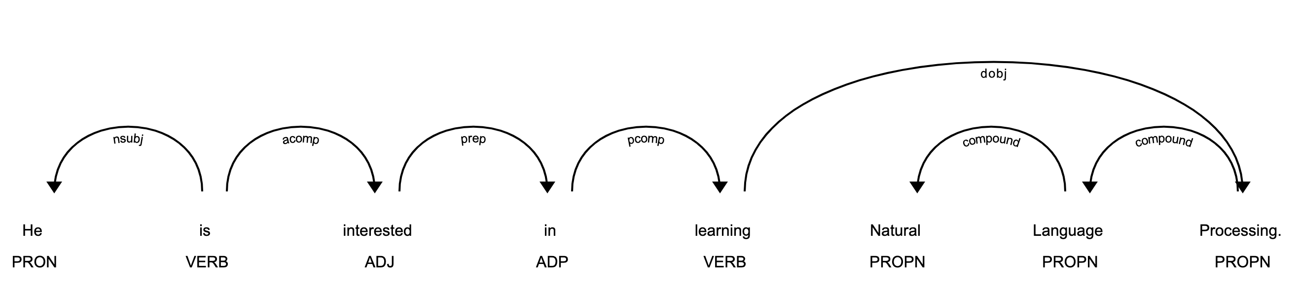
You can use displaCy to find POS tags for tokens:
>>> from spacy import displacy
>>> about_interest_text = ('He is interested in learning'
...     ' Natural Language Processing.')
>>> about_interest_doc = nlp(about_interest_text)
>>> displacy.serve(about_interest_doc, style='dep')
The above code will spin a simple web server. You can see the visualization by opening http://127.0.0.1:5000 in your browser:
In the image above, each token is assigned a POS tag written just below the token.
Note: Here’s how you can use displaCy in a Jupyter notebook:
>>> displacy.render(about_interest_doc, style='dep', jupyter=True)
You can create a preprocessing function that takes text as input and applies the following operations:
A preprocessing function converts text to an analyzable format. It’s necessary for most NLP tasks. Here’s an example:
>>> def is_token_allowed(token):
...     '''
...         Only allow valid tokens which are not stop words
...         and punctuation symbols.
...     '''
...     if (not token or not token.string.strip() or
...         token.is_stop or token.is_punct):
...         return False
...     return True
...
>>> def preprocess_token(token):
...     # Reduce token to its lowercase lemma form
...     return token.lemma_.strip().lower()
...
>>> complete_filtered_tokens = [preprocess_token(token)
...     for token in complete_doc if is_token_allowed(token)]
>>> complete_filtered_tokens
['gus', 'proto', 'python', 'developer', 'currently', 'work',
'london', 'base', 'fintech', 'company', 'interested', 'learn',
'natural', 'language', 'processing', 'developer', 'conference',
'happen', '21', 'july', '2019', 'london', 'title',
'applications', 'natural', 'language', 'processing', 'helpline',
'number', 'available', '+1', '1234567891', 'gus', 'help',
'organize', 'keep', 'organize', 'local', 'python', 'meetup',
'internal', 'talk', 'workplace', 'gus', 'present', 'talk', 'talk',
'introduce', 'reader', 'use', 'case', 'natural', 'language',
'processing', 'fintech', 'apart', 'work', 'passionate', 'music',
'gus', 'learn', 'play', 'piano', 'enrol', 'weekend', 'batch',
'great', 'piano', 'academy', 'great', 'piano', 'academy',
'situate', 'mayfair', 'city', 'london', 'world', 'class',
'piano', 'instructor']
Note that the complete_filtered_tokens does not contain any stop word or punctuation symbols and consists of lemmatized lowercase tokens.
Rule-based matching is one of the steps in extracting information from unstructured text. It’s used to identify and extract tokens and phrases according to patterns (such as lowercase) and grammatical features (such as part of speech).
Rule-based matching can use regular expressions to extract entities (such as phone numbers) from an unstructured text. It’s different from extracting text using regular expressions only in the sense that regular expressions don’t consider the lexical and grammatical attributes of the text.
With rule-based matching, you can extract a first name and a last name, which are always proper nouns:
>>> from spacy.matcher import Matcher
>>> matcher = Matcher(nlp.vocab)
>>> def extract_full_name(nlp_doc):
...     pattern = [{'POS': 'PROPN'}, {'POS': 'PROPN'}]
...     matcher.add('FULL_NAME', None, pattern)
...     matches = matcher(nlp_doc)
...     for match_id, start, end in matches:
...         span = nlp_doc[start:end]
...         return span.text
...
>>> extract_full_name(about_doc)
'Gus Proto'
In this example, pattern is a list of objects that defines the combination of tokens to be matched. Both POS tags in it are PROPN (proper noun). So, the pattern consists of two objects in which the POS tags for both tokens should be PROPN. This pattern is then added to Matcher using FULL_NAME and the the match_id. Finally, matches are obtained with their starting and end indexes.
You can also use rule-based matching to extract phone numbers:
>>> from spacy.matcher import Matcher
>>> matcher = Matcher(nlp.vocab)
>>> conference_org_text = ('There is a developer conference'
...     'happening on 21 July 2019 in London. It is titled'
...     ' "Applications of Natural Language Processing".'
...     ' There is a helpline number available'
...     ' at (123) 456-789')
...
>>> def extract_phone_number(nlp_doc):
...     pattern = [{'ORTH': '('}, {'SHAPE': 'ddd'},
...                {'ORTH': ')'}, {'SHAPE': 'ddd'},
...                {'ORTH': '-', 'OP': '?'},
...                {'SHAPE': 'ddd'}]
...     matcher.add('PHONE_NUMBER', None, pattern)
...     matches = matcher(nlp_doc)
...     for match_id, start, end in matches:
...         span = nlp_doc[start:end]
...         return span.text
...
>>> conference_org_doc = nlp(conference_org_text)
>>> extract_phone_number(conference_org_doc)
'(123) 456-789'
In this example, only the pattern is updated in order to match phone numbers from the previous example. Here, some attributes of the token are also used:
ORTH gives the exact text of the token.SHAPE transforms the token string to show orthographic features.OP defines operators. Using ? as a value means that the pattern is optional, meaning it can match 0 or 1 times.Note: For simplicity, phone numbers are assumed to be of a particular format: (123) 456-789. You can change this depending on your use case.
Rule-based matching helps you identify and extract tokens and phrases according to lexical patterns (such as lowercase) and grammatical features(such as part of speech).
Dependency parsing is the process of extracting the dependency parse of a sentence to represent its grammatical structure. It defines the dependency relationship between headwords and their dependents. The head of a sentence has no dependency and is called the root of the sentence. The verb is usually the head of the sentence. All other words are linked to the headword.
The dependencies can be mapped in a directed graph representation:
Dependency parsing helps you know what role a word plays in the text and how different words relate to each other. It’s also used in shallow parsing and named entity recognition.
Here’s how you can use dependency parsing to see the relationships between words:
>>> piano_text = 'Gus is learning piano'
>>> piano_doc = nlp(piano_text)
>>> for token in piano_doc:
...     print (token.text, token.tag_, token.head.text, token.dep_)
...
Gus NNP learning nsubj
is VBZ learning aux
learning VBG learning ROOT
piano NN learning dobj
In this example, the sentence contains three relationships:
nsubj is the subject of the word. Its headword is a verb.aux is an auxiliary word. Its headword is a verb.dobj is the direct object of the verb. Its headword is a verb.There is a detailed list of relationships with descriptions. You can use displaCy to visualize the dependency tree:
>>> displacy.serve(piano_doc, style='dep')
This code will produce a visualization that can be accessed by opening http://127.0.0.1:5000 in your browser:
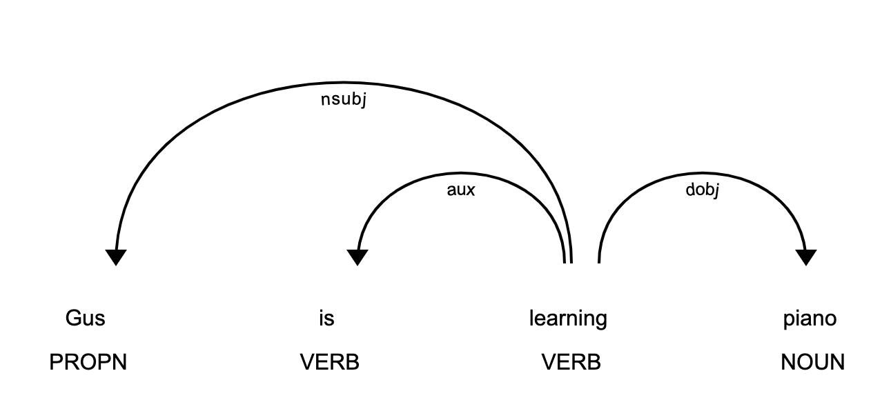
This image shows you that the subject of the sentence is the proper noun Gus and that it has a learn relationship with piano.
The dependency parse tree has all the properties of a tree. This tree contains information about sentence structure and grammar and can be traversed in different ways to extract relationships.
spaCy provides attributes like children, lefts, rights, and subtree to navigate the parse tree:
>>> one_line_about_text = ('Gus Proto is a Python developer'
...     ' currently working for a London-based Fintech company')
>>> one_line_about_doc = nlp(one_line_about_text)
>>> # Extract children of `developer`
>>> print([token.text for token in one_line_about_doc[5].children])
['a', 'Python', 'working']
>>> # Extract previous neighboring node of `developer`
>>> print (one_line_about_doc[5].nbor(-1))
Python
>>> # Extract next neighboring node of `developer`
>>> print (one_line_about_doc[5].nbor())
currently
>>> # Extract all tokens on the left of `developer`
>>> print([token.text for token in one_line_about_doc[5].lefts])
['a', 'Python']
>>> # Extract tokens on the right of `developer`
>>> print([token.text for token in one_line_about_doc[5].rights])
['working']
>>> # Print subtree of `developer`
>>> print (list(one_line_about_doc[5].subtree))
[a, Python, developer, currently, working, for, a, London, -,
based, Fintech, company]
You can construct a function that takes a subtree as an argument and returns a string by merging words in it:
>>> def flatten_tree(tree):
...     return ''.join([token.text_with_ws for token in list(tree)]).strip()
...
>>> # Print flattened subtree of `developer`
>>> print (flatten_tree(one_line_about_doc[5].subtree))
a Python developer currently working for a London-based Fintech company
You can use this function to print all the tokens in a subtree.
Shallow parsing, or chunking, is the process of extracting phrases from unstructured text. Chunking groups adjacent tokens into phrases on the basis of their POS tags. There are some standard well-known chunks such as noun phrases, verb phrases, and prepositional phrases.
A noun phrase is a phrase that has a noun as its head. It could also include other kinds of words, such as adjectives, ordinals, determiners. Noun phrases are useful for explaining the context of the sentence. They help you infer what is being talked about in the sentence.
spaCy has the property noun_chunks on Doc object. You can use it to extract noun phrases:
>>> conference_text = ('There is a developer conference'
...     ' happening on 21 July 2019 in London.')
>>> conference_doc = nlp(conference_text)
>>> # Extract Noun Phrases
>>> for chunk in conference_doc.noun_chunks:
...     print (chunk)
...
a developer conference
21 July
London
By looking at noun phrases, you can get information about your text. For example, a developer conference indicates that the text mentions a conference, while the date 21 July lets you know that conference is scheduled for 21 July. You can figure out whether the conference is in the past or the future. London tells you that the conference is in London.
A verb phrase is a syntactic unit composed of at least one verb. This verb can be followed by other chunks, such as noun phrases. Verb phrases are useful for understanding the actions that nouns are involved in.
spaCy has no built-in functionality to extract verb phrases, so you’ll need a library called textacy:
Note:
You can use pip to install textacy:
$ pip install textacy
Now that you have textacy installed, you can use it to extract verb phrases based on grammar rules:
>>> import textacy
>>> about_talk_text = ('The talk will introduce reader about Use'
...                    ' cases of Natural Language Processing in'
...                    ' Fintech')
>>> pattern = r'(<VERB>?<ADV>*<VERB>+)'
>>> about_talk_doc = textacy.make_spacy_doc(about_talk_text,
...                                         lang='en_core_web_sm')
>>> verb_phrases = textacy.extract.pos_regex_matches(about_talk_doc, pattern)
>>> # Print all Verb Phrase
>>> for chunk in verb_phrases:
...     print(chunk.text)
...
will introduce
>>> # Extract Noun Phrase to explain what nouns are involved
>>> for chunk in about_talk_doc.noun_chunks:
...     print (chunk)
...
The talk
reader
Use cases
Natural Language Processing
Fintech
In this example, the verb phrase introduce indicates that something will be introduced. By looking at noun phrases, you can see that there is a talk that will introduce the reader to use cases of Natural Language Processing or Fintech.
The above code extracts all the verb phrases using a regular expression pattern of POS tags. You can tweak the pattern for verb phrases depending upon your use case.
Note: In the previous example, you could have also done dependency parsing to see what the relationships between the words were.
Named Entity Recognition (NER) is the process of locating named entities in unstructured text and then classifying them into pre-defined categories, such as person names, organizations, locations, monetary values, percentages, time expressions, and so on.
You can use NER to know more about the meaning of your text. For example, you could use it to populate tags for a set of documents in order to improve the keyword search. You could also use it to categorize customer support tickets into relevant categories.
spaCy has the property ents on Doc objects. You can use it to extract named entities:
>>> piano_class_text = ('Great Piano Academy is situated'
...     ' in Mayfair or the City of London and has'
...     ' world-class piano instructors.')
>>> piano_class_doc = nlp(piano_class_text)
>>> for ent in piano_class_doc.ents:
...     print(ent.text, ent.start_char, ent.end_char,
...           ent.label_, spacy.explain(ent.label_))
...
Great Piano Academy 0 19 ORG Companies, agencies, institutions, etc.
Mayfair 35 42 GPE Countries, cities, states
the City of London 46 64 GPE Countries, cities, states
In the above example, ent is a Span object with various attributes:
text gives the Unicode text representation of the entity.start_char denotes the character offset for the start of the entity.end_char denotes the character offset for the end of the entity.label_ gives the label of the entity.spacy.explain gives descriptive details about an entity label. The spaCy model has a pre-trained list of entity classes. You can use displaCy to visualize these entities:
>>> displacy.serve(piano_class_doc, style='ent')
If you open http://127.0.0.1:5000 in your browser, then you can see the visualization:

You can use NER to redact people’s names from a text. For example, you might want to do this in order to hide personal information collected in a survey. You can use spaCy to do that:
>>> survey_text = ('Out of 5 people surveyed, James Robert,'
...                ' Julie Fuller and Benjamin Brooks like'
...                ' apples. Kelly Cox and Matthew Evans'
...                ' like oranges.')
...
>>> def replace_person_names(token):
...     if token.ent_iob != 0 and token.ent_type_ == 'PERSON':
...         return '[REDACTED] '
...     return token.string
...
>>> def redact_names(nlp_doc):
...     for ent in nlp_doc.ents:
...         ent.merge()
...     tokens = map(replace_person_names, nlp_doc)
...     return ''.join(tokens)
...
>>> survey_doc = nlp(survey_text)
>>> redact_names(survey_doc)
'Out of 5 people surveyed, [REDACTED] , [REDACTED] and'
' [REDACTED] like apples. [REDACTED] and [REDACTED]'
' like oranges.'
In this example, replace_person_names() uses ent_iob. It gives the IOB code of the named entity tag using inside-outside-beginning (IOB) tagging. Here, it can assume a value other than zero, because zero means that no entity tag is set.
spaCy is a powerful and advanced library that is gaining huge popularity for NLP applications due to its speed, ease of use, accuracy, and extensibility. Congratulations! You now know:
[ Improve Your Python With 🐍 Python Tricks 💌 – Get a short & sweet Python Trick delivered to your inbox every couple of days. >> Click here to learn more and see examples ]
# datePublished: #Mon Sep 2 14:00:00 2019# dateUpdated: #Mon Sep 2 14:00:00 2019# # Person begin #################### name: #Real Python# # Person end ###################### # Item end ######################## # Item begin ###################### id: #https://realpython.com/pycharm-guide/# title: #PyCharm for Productive Python Development (Guide)# link: #https://realpython.com/pycharm-guide/# description: #In this step-by-step tutorial, you'll learn how you can use PyCharm to be a more productive Python developer. PyCharm makes debugging and visualization easy so you can focus on business logic and just get the job done.# content: #As a programmer, you should be focused on the business logic and creating useful applications for your users. In doing that, PyCharm by JetBrains saves you a lot of time by taking care of the routine and by making a number of other tasks such as debugging and visualization easy.
In this article, you’ll learn about:
This article assumes that you’re familiar with Python development and already have some form of Python installed on your system. Python 3.6 will be used for this tutorial. Screenshots and demos provided are for macOS. Because PyCharm runs on all major platforms, you may see slightly different UI elements and may need to modify certain commands.
Note:
PyCharm comes in three editions:
For more details on their differences, check out the PyCharm Editions Comparison Matrix by JetBrains. The company also has special offers for students, teachers, open source projects, and other cases.
Clone Repo: Click here to clone the repo you'll use to explore the project-focused features of PyCharm in this tutorial.
This article will use PyCharm Community Edition 2019.1 as it’s free and available on every major platform. Only the section about the professional features will use PyCharm Professional Edition 2019.1.
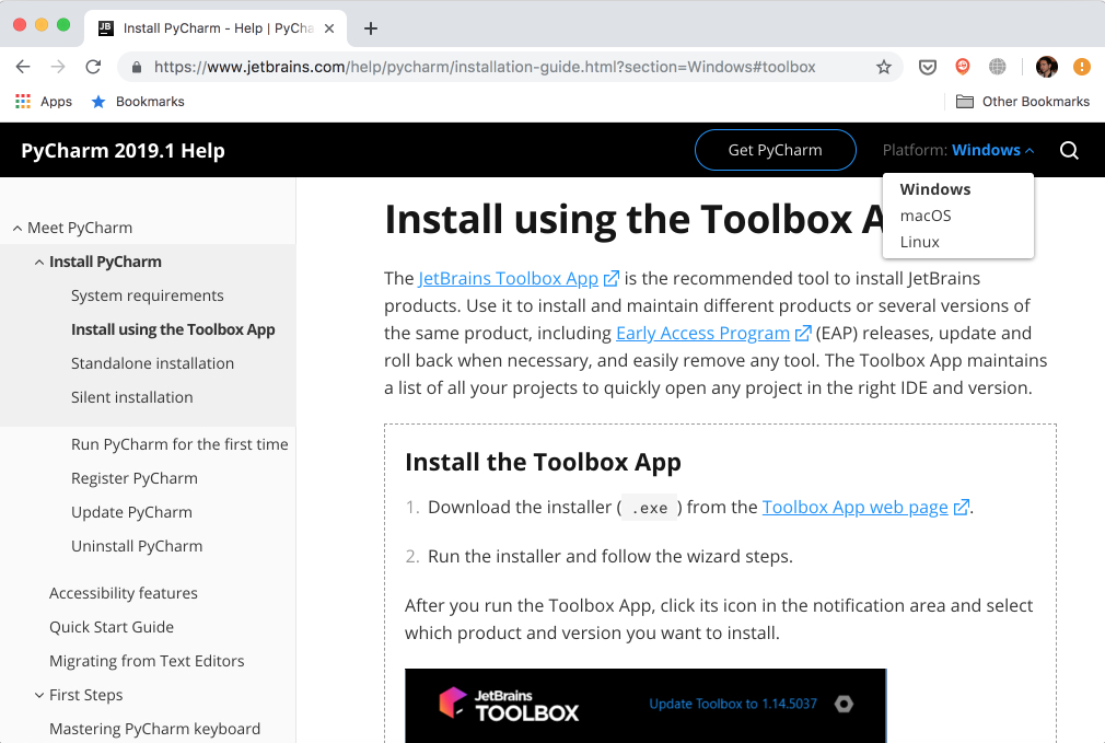
The recommended way of installing PyCharm is with the JetBrains Toolbox App. With its help, you’ll be able to install different JetBrains products or several versions of the same product, update, rollback, and easily remove any tool when necessary. You’ll also be able to quickly open any project in the right IDE and version.
To install the Toolbox App, refer to the documentation by JetBrains. It will automatically give you the right instructions depending on your OS. In case it didn’t recognize your OS correctly, you can always find it from the drop down list on the top right section:
After installing, launch the app and accept the user agreement. Under the Tools tab, you’ll see a list of available products. Find PyCharm Community there and click Install:
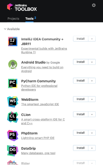
Voilà! You have PyCharm available on your machine. If you don’t want to use the Toolbox app, then you can also do a stand-alone installation of PyCharm.
Launch PyCharm, and you’ll see the import settings popup:
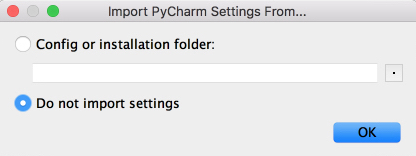
PyCharm will automatically detect that this is a fresh install and choose Do not import settings for you. Click OK, and PyCharm will ask you to select a keymap scheme. Leave the default and click Next: UI Themes on the bottom right:
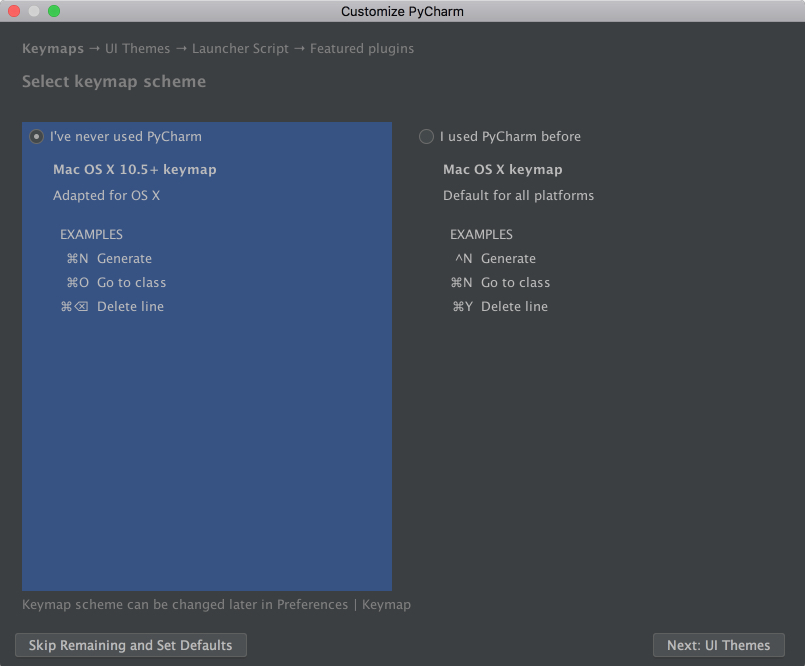
PyCharm will then ask you to choose a dark theme called Darcula or a light theme. Choose whichever you prefer and click Next: Launcher Script:
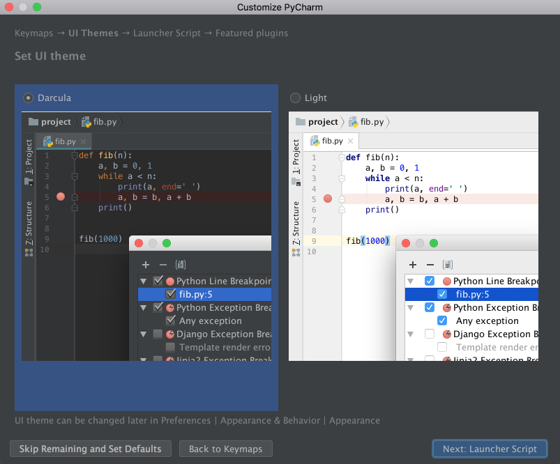
I’ll be using the dark theme Darcula throughout this tutorial. You can find and install other themes as plugins, or you can also import them.
On the next page, leave the defaults and click Next: Featured plugins. There, PyCharm will show you a list of plugins you may want to install because most users like to use them. Click Start using PyCharm, and now you are ready to write some code!
In PyCharm, you do everything in the context of a project. Thus, the first thing you need to do is create one.
After installing and opening PyCharm, you are on the welcome screen. Click Create New Project, and you’ll see the New Project popup:
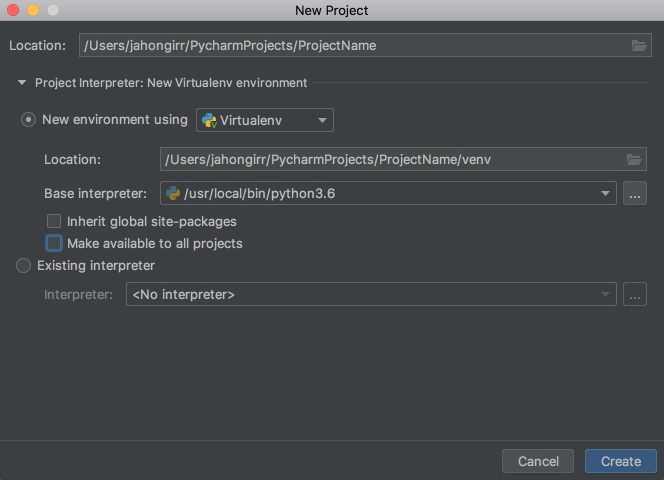
Specify the project location and expand the Project Interpreter drop down. Here, you have options to create a new project interpreter or reuse an existing one. Choose New environment using. Right next to it, you have a drop down list to select one of Virtualenv, Pipenv, or Conda, which are the tools that help to keep dependencies required by different projects separate by creating isolated Python environments for them.
You are free to select whichever you like, but Virtualenv is used for this tutorial. If you choose to, you can specify the environment location and choose the base interpreter from the list, which is a list of Python interpreters (such as Python2.7 and Python3.6) installed on your system. Usually, the defaults are fine. Then you have to select boxes to inherit global site-packages to your new environment and make it available to all other projects. Leave them unselected.
Click Create on the bottom right and you will see the new project created:
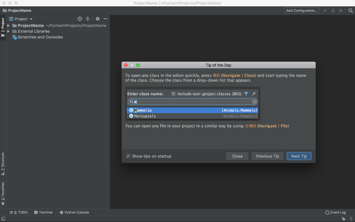
You will also see a small Tip of the Day popup where PyCharm gives you one trick to learn at each startup. Go ahead and close this popup.
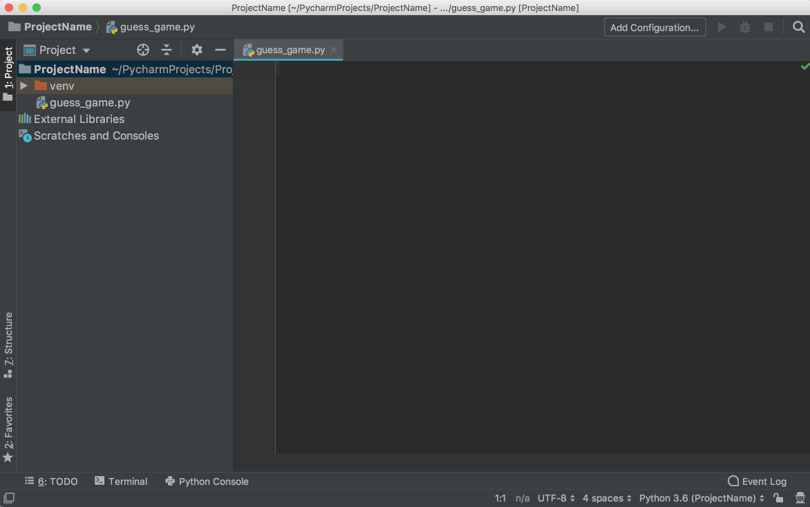
It is now time to start a new Python program. Type Cmd+N if you are on Mac or Alt+Ins if you are on Windows or Linux. Then, choose Python File. You can also select File → New from the menu. Name the new file guess_game.py and click OK. You will see a PyCharm window similar to the following:
For our test code, let’s quickly code up a simple guessing game in which the program chooses a number that the user has to guess. For every guess, the program will tell if the user’s guess was smaller or bigger than the secret number. The game ends when the user guesses the number. Here’s the code for the game:
 1 from random import randint
 2
 3 def play():
 4     random_int = randint(0, 100)
 5
 6     while True:
 7         user_guess = int(input("What number did we guess (0-100)?"))
 8
 9         if user_guess == randint:
10             print(f"You found the number ({random_int}). Congrats!")
11             break
12
13         if user_guess < random_int:
14             print("Your number is less than the number we guessed.")
15             continue
16
17         if user_guess > random_int:
18             print("Your number is more than the number we guessed.")
19             continue
20
21
22 if __name__ == '__main__':
23     play()
Type this code directly rather than copying and pasting. You’ll see something like this:

As you can see, PyCharm provides Intelligent Coding Assistance with code completion, code inspections, on-the-fly error highlighting, and quick-fix suggestions. In particular, note how when you typed main and then hit tab, PyCharm auto-completed the whole main clause for you.
Also note how, if you forget to type if before the condition, append .if, and then hit Tab, PyCharm fixes the if clause for you. The same is true with True.while. That’s PyCharm’s Postfix completions working for you to help reduce backward caret jumps.
Now that you’ve coded up the game, it’s time for you to run it.
You have three ways of running this program:
__main__ clause, you can click on the little green arrow to the left of the __main__ clause and choose Run ‘guess_game’ from there.Use any one of the options above to run the program, and you’ll see the Run Tool pane appear at the bottom of the window, with your code output showing:
Play the game for a little bit to see if you can find the number guessed. Pro tip: start with 50.
Did you find the number? If so, you may have seen something weird after you found the number. Instead of printing the congratulations message and exiting, the program seems to start over. That’s a bug right there. To discover why the program starts over, you’ll now debug the program.
First, place a breakpoint by clicking on the blank space to the left of line number 8:
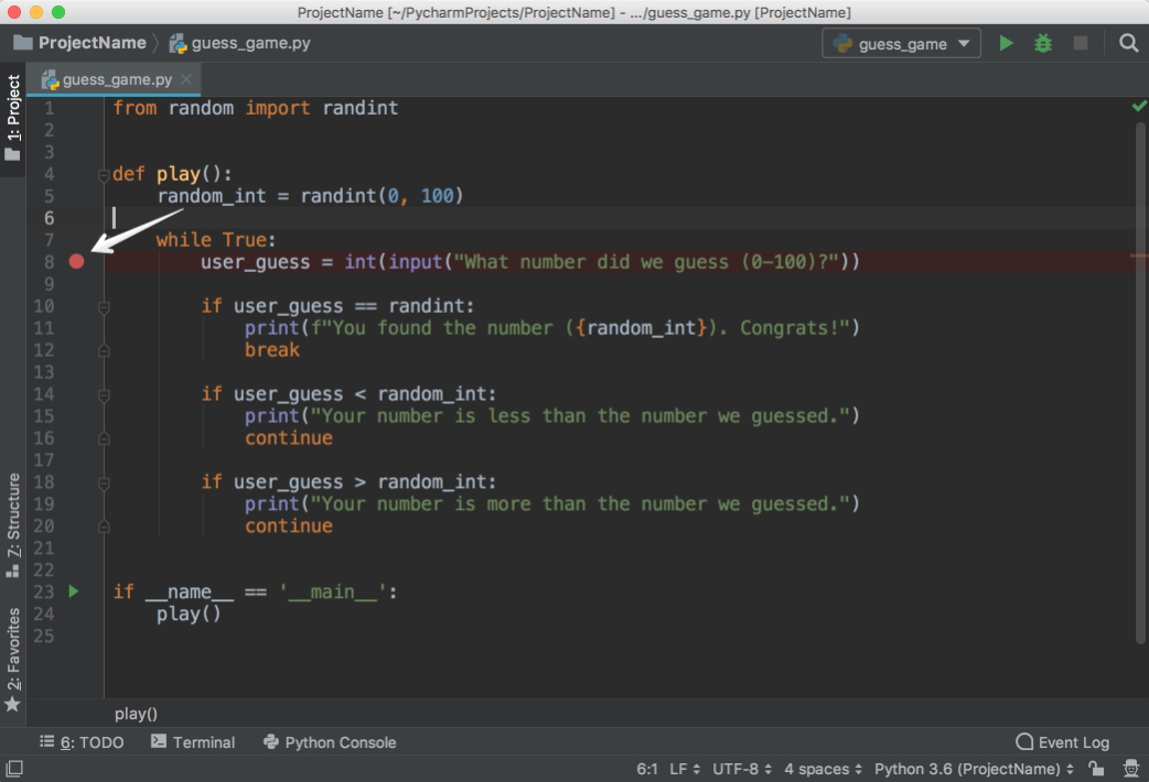
This will be the point where the program will be suspended, and you can start exploring what went wrong from there on. Next, choose one of the following three ways to start debugging:
__main__ clause and choose Debug ‘guess_game from there.Afterwards, you’ll see a Debug window open at the bottom:
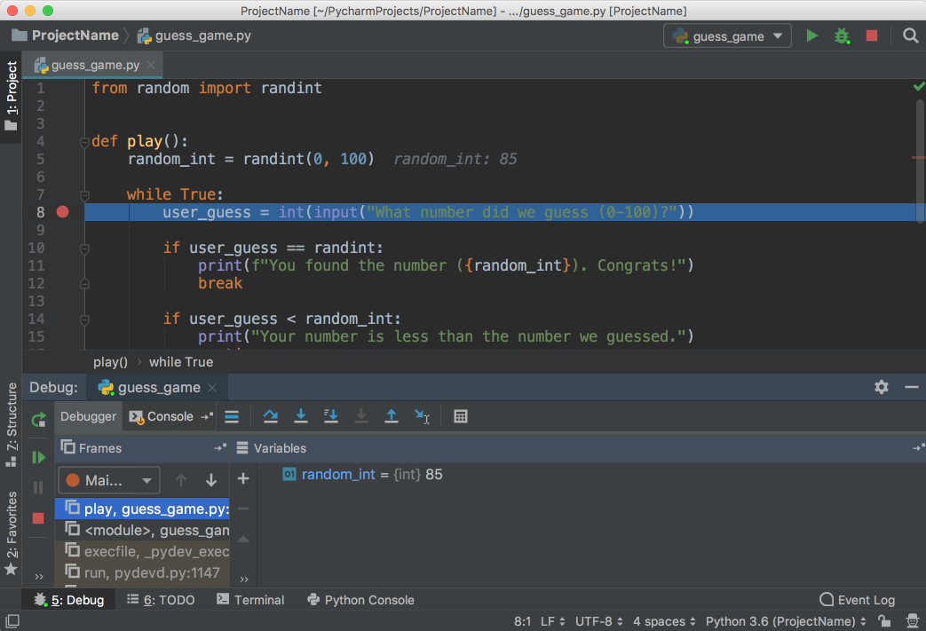
Follow the steps below to debug the program:
Notice that the current line is highlighted in blue.
See that random_int and its value are listed in the Debug window. Make a note of this number. (In the picture, the number is 85.)
Hit F8 to execute the current line and step over to the next one. You can also use F7 to step into the function in the current line, if necessary. As you continue executing the statements, the changes in the variables will be automatically reflected in the Debugger window.
Notice that there is the Console tab right next to the Debugger tab that opened. This Console tab and the Debugger tab are mutually exclusive. In the Console tab, you will be interacting with your program, and in the Debugger tab you will do the debugging actions.
Switch to the Console tab to enter your guess.
Type the number shown, and then hit Enter.
Switch back to the Debugger tab.
Hit F8 again to evaluate the if statement. Notice that you are now on line 14. But wait a minute! Why didn’t it go to the line 11? The reason is that the if statement on line 10 evaluated to False. But why did it evaluate to False when you entered the number that was chosen?
Look carefully at line 10 and notice that we are comparing user_guess with the wrong thing. Instead of comparing it with random_int, we are comparing it with randint, the function that was imported from the random package.
Change it to random_int, restart the debugging, and follow the same steps again. You will see that, this time, it will go to line 11, and line 10 will evaluate to True:

Congratulations! You fixed the bug.
No application is reliable without unit tests. PyCharm helps you write and run them very quickly and comfortably. By default, unittest is used as the test runner, but PyCharm also supports other testing frameworks such as pytest, nose, doctest, tox, and trial. You can, for example, enable pytest for your project like this:
pytest in the Default test runner field.For this example, we’ll be using the default test runner unittest.
In the same project, create a file called calculator.py and put the following Calculator class in it:
 1 class Calculator:
 2     def add(self, a, b):
 3         return a + b
 4
 5     def multiply(self, a, b):
 6         return a * b
PyCharm makes it very easy to create tests for your existing code. With the calculator.py file open, execute any one of the following that you like:
Choose Create New Test…, and you will see the following window:
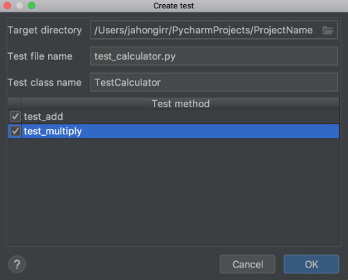
Leave the defaults of Target directory, Test file name, and Test class name. Select both of the methods and click OK. Voila! PyCharm automatically created a file called test_calculator.py and created the following stub tests for you in it:
 1 from unittest import TestCase
 2
 3 class TestCalculator(TestCase):
 4     def test_add(self):
 5         self.fail()
 6
 7     def test_multiply(self):
 8         self.fail()
Run the tests using one of the methods below:
You’ll see the tests window open on the bottom with all the tests failing:
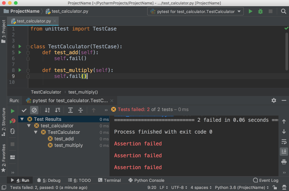
Notice that you have the hierarchy of the test results on the left and the output of the terminal on the right.
Now, implement test_add by changing the code to the following:
 1 from unittest import TestCase
 2
 3 from calculator import Calculator
 4
 5 class TestCalculator(TestCase):
 6     def test_add(self):
 7         self.calculator = Calculator()
 8         self.assertEqual(self.calculator.add(3, 4), 7)
 9
10     def test_multiply(self):
11         self.fail()
Run the tests again, and you’ll see that one test passed and the other failed. Explore the options to show passed tests, to show ignored tests, to sort tests alphabetically, and to sort tests by duration:
Note that the sleep(0.1) method that you see in the GIF above is intentionally used to make one of the tests slower so that sorting by duration works.
These single file projects are great for examples, but you’ll often work on much larger projects over a longer period of time. In this section, you’ll take a look at how PyCharm works with a larger project.
To explore the project-focused features of PyCharm, you’ll use the Alcazar web framework that was built for learning purposes. To continue following along, clone the repo locally:
Clone Repo: Click here to clone the repo you'll use to explore the project-focused features of PyCharm in this tutorial.
Once you have a project locally, open it in PyCharm using one of the following methods:
After either of these steps, find the folder containing the project on your computer and open it.
If this project contains a virtual environment, then PyCharm will automatically use this virtual environment and make it the project interpreter.
If you need to configure a different virtualenv, then open Preferences on Mac by pressing Cmd+, or Settings on Windows or Linux by pressing Ctrl+Alt+S and find the Project: ProjectName section. Open the drop-down and choose Project Interpreter:
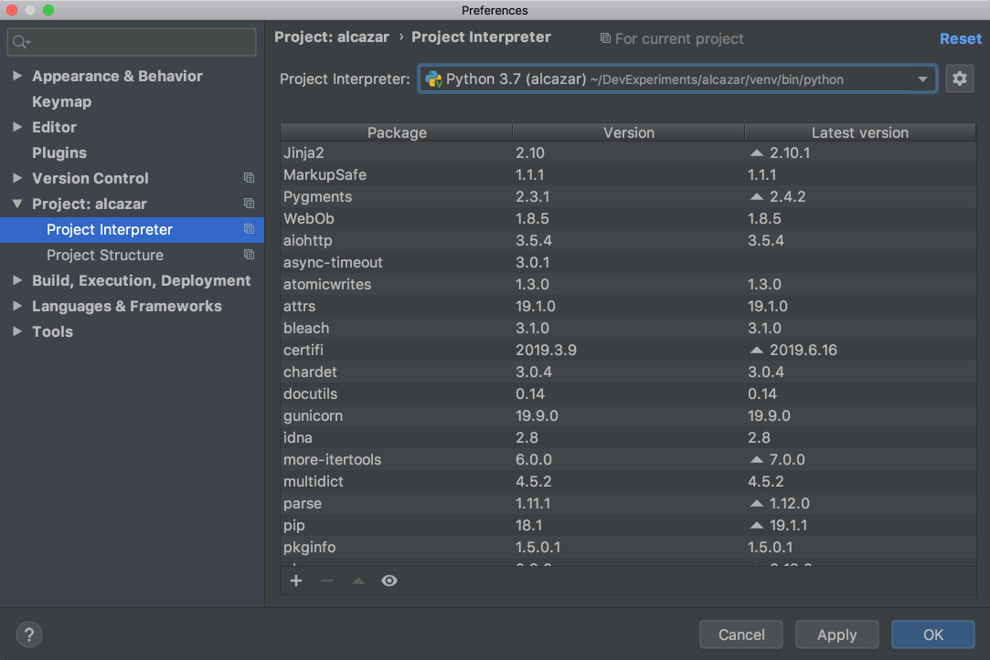
Choose the virtualenv from the drop-down list. If it’s not there, then click on the settings button to the right of the drop-down list and then choose Add…. The rest of the steps should be the same as when we were creating a new project.
In a big project where it’s difficult for a single person to remember where everything is located, it’s very important to be able to quickly navigate and find what you looking for. PyCharm has you covered here as well. Use the project you opened in the section above to practice these shortcuts:
As for the navigation, the following shortcuts may save you a lot of time:
For more details, see the official documentation.
Version control systems such as Git and Mercurial are some of the most important tools in the modern software development world. So, it is essential for an IDE to support them. PyCharm does that very well by integrating with a lot of popular VC systems such as Git (and Github), Mercurial, Perforce and, Subversion.
Note: Git is used for the following examples.
To enable VCS integration. Go to VCS → VCS Operations Popup… from the menu on the top or press Ctrl+V on Mac or Alt+` on Windows or Linux. Choose Enable Version Control Integration…. You’ll see the following window open:
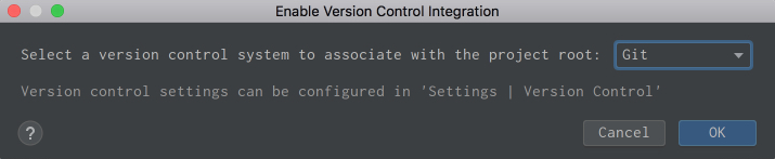
Choose Git from the drop down list, click OK, and you have VCS enabled for your project. Note that if you opened an existing project that has version control enabled, then PyCharm will see that and automatically enable it.
Now, if you go to the VCS Operations Popup…, you’ll see a different popup with the options to do git add, git stash, git branch, git commit, git push and more:
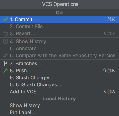
If you can’t find what you need, you can most probably find it by going to VCS from the top menu and choosing Git, where you can even create and view pull requests.
These are two features of VCS integration in PyCharm that I personally use and enjoy a lot! Let’s say you have finished your work and want to commit it. Go to VCS → VCS Operations Popup… → Commit… or press Cmd+K on Mac or Ctrl+K on Windows or Linux. You’ll see the following window open:

In this window, you can do the following:
It can feel magical and fast, especially if you’re used to doing everything manually on the command line.
When you work in a team, merge conflicts do happen. When somebody commits changes to a file that you’re working on, but their changes overlap with yours because both of you changed the same lines, then VCS will not be able to figure out if it should choose your changes or those of your teammate. So you’ll get these unfortunate arrows and symbols:
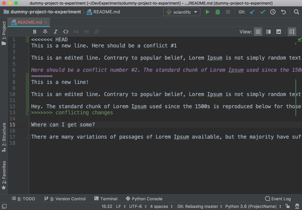
This looks strange, and it’s difficult to figure out which changes should be deleted and which ones should stay. PyCharm to the rescue! It has a much nicer and cleaner way of resolving conflicts. Go to VCS in the top menu, choose Git and then Resolve conflicts…. Choose the file whose conflicts you want to resolve and click on Merge. You will see the following window open:
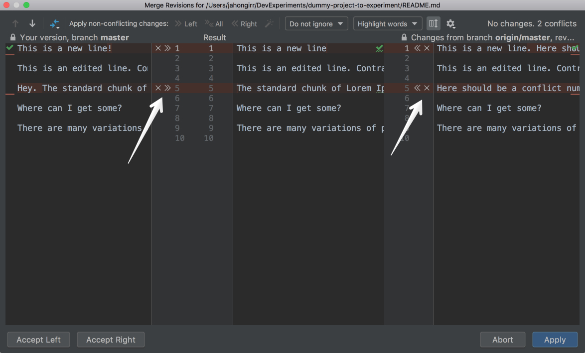
On the left column, you will see your changes. On the right one, the changes made by your teammate. Finally, in the middle column, you will see the result. The conflicting lines are highlighted, and you can see a little X and >>/<< right beside those lines. Press the arrows to accept the changes and the X to decline. After you resolve all those conflicts, click the Apply button:

In the GIF above, for the first conflicting line, the author declined his own changes and accepted those of his teammates. Conversely, the author accepted his own changes and declined his teammates’ for the second conflicting line.
There’s a lot more that you can do with the VCS integration in PyCharm. For more details, see this documentation.
You can find almost everything you need for development in PyCharm. If you can’t, there is most probably a plugin that adds that functionality you need to PyCharm. For example, they can:
For instance, IdeaVim adds Vim emulation to PyCharm. If you like Vim, this can be a pretty good combination.
Material Theme UI changes the appearance of PyCharm to a Material Design look and feel:
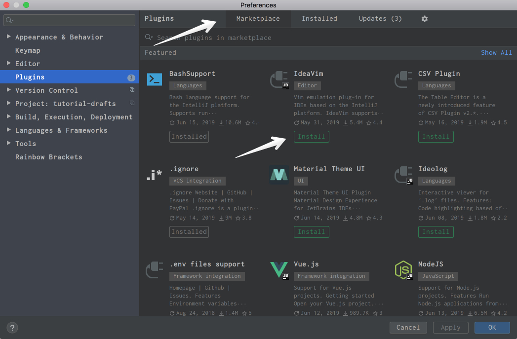
Vue.js adds support for Vue.js projects. Markdown provides the capability to edit Markdown files within the IDE and see the rendered HTML in a live preview. You can find and install all of the available plugins by going to the Preferences → Plugins on Mac or Settings → Plugins on Windows or Linux, under the Marketplace tab:
If you can’t find what you need, you can even develop your own plugin.
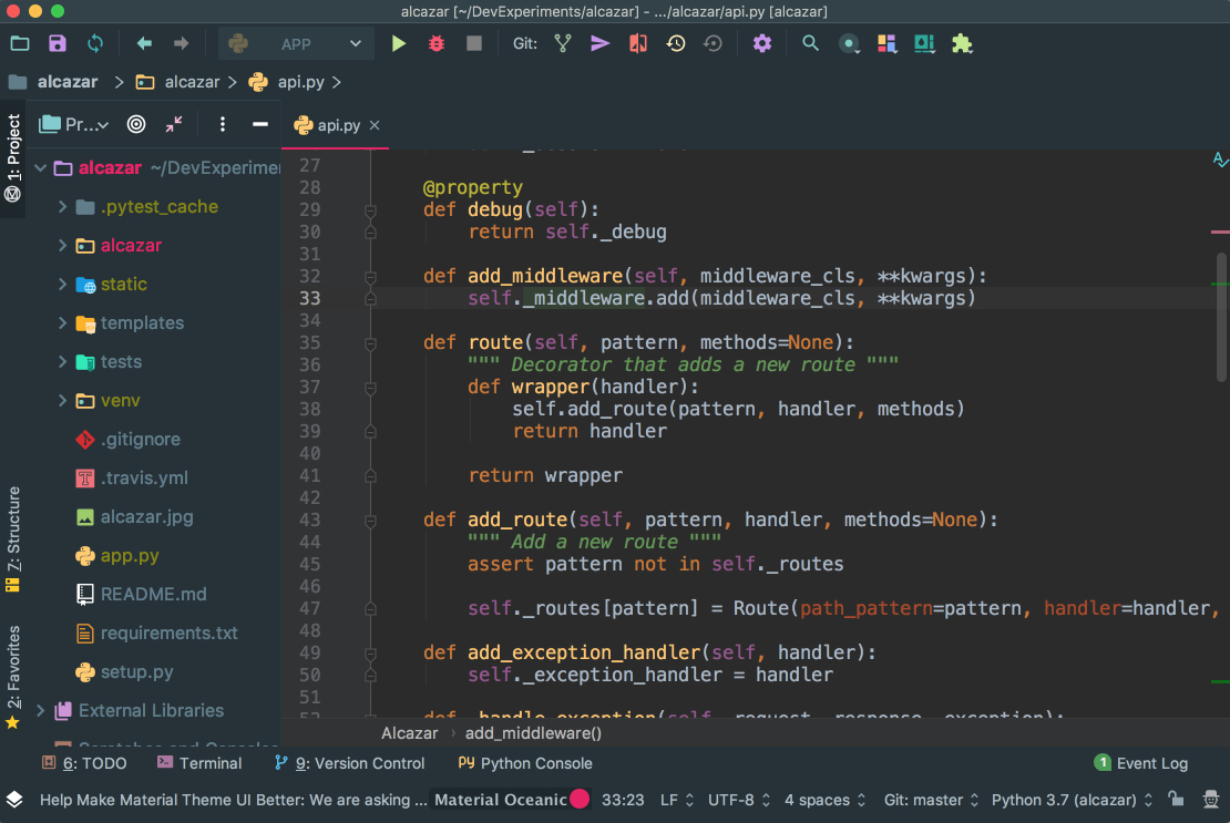
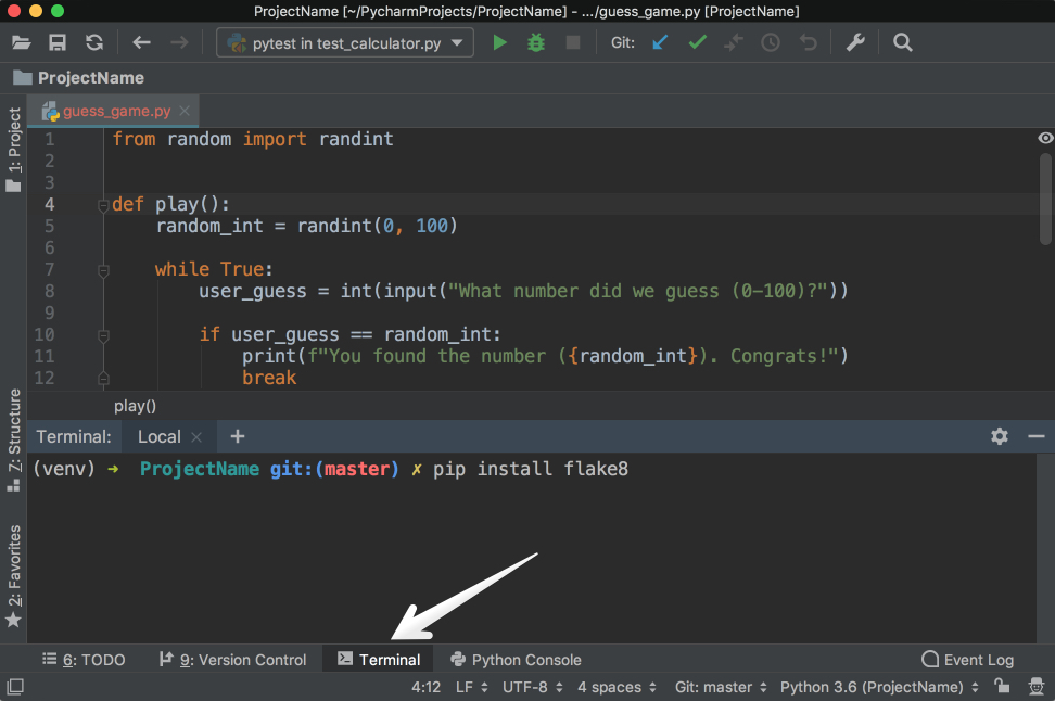
If you can’t find the right plugin and don’t want to develop your own because there’s already a package in PyPI, then you can add it to PyCharm as an external tool. Take Flake8, the code analyzer, as an example.
First, install flake8 in your virtualenv with pip install flake8 in the Terminal app of your choice. You can also use the one integrated into PyCharm:
Then, go to Preferences → Tools on Mac or Settings → Tools on Windows/Linux, and then choose External Tools. Then click on the little + button at the bottom (1). In the new popup window, insert the details as shown below and click OK for both windows:
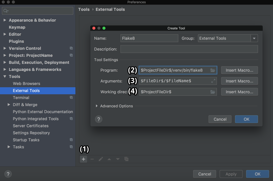
Here, Program (2) refers to the Flake8 executable that can be found in the folder /bin of your virtual environment. Arguments (3) refers to which file you want to analyze with the help of Flake8. Working directory is the directory of your project.
You could hardcode the absolute paths for everything here, but that would mean that you couldn’t use this external tool in other projects. You would be able to use it only inside one project for one file.
So you need to use something called Macros. Macros are basically variables in the format of $name$ that change according to your context. For example, $FileName$ is first.py when you’re editing first.py, and it is second.py when you’re editing second.py. You can see their list and insert any of them by clicking on the Insert Macro… buttons. Because you used macros here, the values will change according to the project you’re currently working on, and Flake8 will continue to do its job properly.
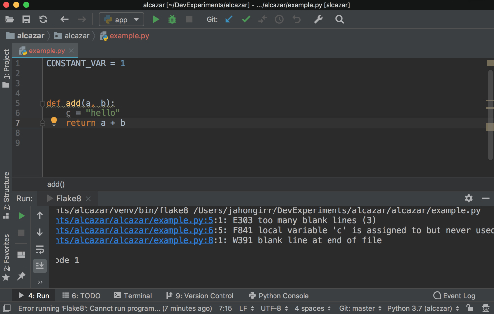
In order to use it, create a file example.py and put the following code in it:
 1 CONSTANT_VAR = 1
 2
 3
 4
 5 def add(a, b):
 6     c = "hello"
 7     return a + b
It deliberately breaks some of the Flake8 rules. Right-click the background of this file. Choose External Tools and then Flake8. Voilà! The output of the Flake8 analysis will appear at the bottom:
In order to make it even better, you can add a shortcut for it. Go to Preferences on Mac or to Settings on Windows or Linux. Then, go to Keymap → External Tools → External Tools. Double-click Flake8 and choose Add Keyboard Shortcut. You’ll see this window:
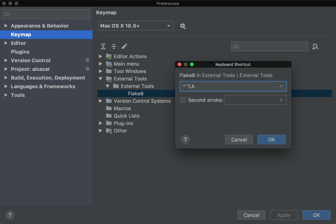
In the image above, the shortcut is Ctrl+Alt+A for this tool. Add your preferred shortcut in the textbox and click OK for both windows. Now you can now use that shortcut to analyze the file you’re currently working on with Flake8.
PyCharm Professional is a paid version of PyCharm with more out-of-the-box features and integrations. In this section, you’ll mainly be presented with overviews of its main features and links to the official documentation, where each feature is discussed in detail. Remember that none of the following features is available in the Community edition.
PyCharm has extensive support for Django, one of the most popular and beloved Python web frameworks. To make sure that it’s enabled, do the following:
Now that you’ve enabled Django support, your Django development journey will be a lot easier in PyCharm:
django-admin startproject mysite.manage.py commands directly inside PyCharm. For more details on Django support, see the official documentation.
Modern database development is a complex task with many supporting systems and workflows. That’s why JetBrains, the company behind PyCharm, developed a standalone IDE called DataGrip for that. It’s a separate product from PyCharm with a separate license.
Luckily, PyCharm supports all the features that are available in DataGrip through a plugin called Database tools and SQL, which is enabled by default. With the help of it, you can query, create and manage databases whether they’re working locally, on a server, or in the cloud. The plugin supports MySQL, PostgreSQL, Microsoft SQL Server, SQLite, MariaDB, Oracle, Apache Cassandra, and others. For more information on what you can do with this plugin, check out the comprehensive documentation on the database support.
Django Channels, asyncio, and the recent frameworks like Starlette are examples of a growing trend in asynchronous Python programming. While it’s true that asynchronous programs do bring a lot of benefits to the table, it’s also notoriously hard to write and debug them. In such cases, Thread Concurrency Visualization can be just what the doctor ordered because it helps you take full control over your multi-threaded applications and optimize them.
Check out the comprehensive documentation of this feature for more details.
Speaking of optimization, profiling is another technique that you can use to optimize your code. With its help, you can see which parts of your code are taking most of the execution time. A profiler runs in the following order of priority:
If you don’t have vmprof or yappi installed, then it’ll fall back to the standard cProfile. It’s well-documented, so I won’t rehash it here.
Python is not only a language for general and web programming. It also emerged as the best tool for data science and machine learning over these last years thanks to libraries and tools like NumPy, SciPy, scikit-learn, Matplotlib, Jupyter, and more. With such powerful libraries available, you need a powerful IDE to support all the functions such as graphing and analyzing those libraries have. PyCharm provides everything you need as thoroughly documented here.
One common cause of bugs in many applications is that development and production environments differ. Although, in most cases, it’s not possible to provide an exact copy of the production environment for development, pursuing it is a worthy goal.
With PyCharm, you can debug your application using an interpreter that is located on the other computer, such as a Linux VM. As a result, you can have the same interpreter as your production environment to fix and avoid many bugs resulting from the difference between development and production environments. Make sure to check out the official documentation to learn more.
PyCharm is one of best, if not the best, full-featured, dedicated, and versatile IDEs for Python development. It offers a ton of benefits, saving you a lot of time by helping you with routine tasks. Now you know how to be productive with it!
In this article, you learned about a lot, including:
If there’s anything you’d like to ask or share, please reach out in the comments below. There’s also a lot more information at the PyCharm website for you to explore.
Clone Repo: Click here to clone the repo you'll use to explore the project-focused features of PyCharm in this tutorial.
[ Improve Your Python With 🐍 Python Tricks 💌 – Get a short & sweet Python Trick delivered to your inbox every couple of days. >> Click here to learn more and see examples ]
# datePublished: #Wed Aug 28 14:00:00 2019# dateUpdated: #Wed Aug 28 14:00:00 2019# # Person begin #################### name: #Real Python# # Person end ###################### # Item end ######################## # Item begin ###################### id: #https://realpython.com/courses/python-lambda-functions/# title: #How to Use Python Lambda Functions# link: #https://realpython.com/courses/python-lambda-functions/# description: #In this step-by-step course, you'll learn about Python lambda functions. You'll see how they compare with regular functions and how you can use them in accordance with best practices.# content: #Python and other languages like Java, C#, and even C++ have had lambda functions added to their syntax, whereas languages like LISP or the ML family of languages, Haskell, OCaml, and F#, use lambdas as a core concept. Python lambdas are little, anonymous functions, subject to a more restrictive but more concise syntax than regular Python functions.
By the end of this course, you’ll know:
This course is mainly for intermediate to experienced Python programmers, but it is accessible to any curious minds with interest in programming. All the examples included in this tutorial have been tested with Python 3.7.
[ Improve Your Python With 🐍 Python Tricks 💌 – Get a short & sweet Python Trick delivered to your inbox every couple of days. >> Click here to learn more and see examples ]
# datePublished: #Tue Aug 27 14:00:00 2019# dateUpdated: #Tue Aug 27 14:00:00 2019# # Person begin #################### name: #Real Python# # Person end ###################### # Item end ######################## # Item begin ###################### id: #https://realpython.com/openpyxl-excel-spreadsheets-python/# title: #A Guide to Excel Spreadsheets in Python With openpyxl# link: #https://realpython.com/openpyxl-excel-spreadsheets-python/# description: #In this step-by-step tutorial, you'll learn how to handle spreadsheets in Python using the openpyxl package. You'll learn how to manipulate Excel spreadsheets, extract information from spreadsheets, create simple or more complex spreadsheets, including adding styles, charts, and so on.# content: #Excel spreadsheets are one of those things you might have to deal with at some point. Either it’s because your boss loves them or because marketing needs them, you might have to learn how to work with spreadsheets, and that’s when knowing openpyxl comes in handy!
Spreadsheets are a very intuitive and user-friendly way to manipulate large datasets without any prior technical background. That’s why they’re still so commonly used today.
In this article, you’ll learn how to use openpyxl to:
This article is written for intermediate developers who have a pretty good knowledge of Python data structures, such as dicts and lists, but also feel comfortable around OOP and more intermediate level topics.
Download Dataset: Click here to download the dataset for the openpyxl exercise you'll be following in this tutorial.
If you ever get asked to extract some data from a database or log file into an Excel spreadsheet, or if you often have to convert an Excel spreadsheet into some more usable programmatic form, then this tutorial is perfect for you. Let’s jump into the openpyxl caravan!
First things first, when would you need to use a package like openpyxl in a real-world scenario? You’ll see a few examples below, but really, there are hundreds of possible scenarios where this knowledge could come in handy.
You are responsible for tech in an online store company, and your boss doesn’t want to pay for a cool and expensive CMS system.
Every time they want to add new products to the online store, they come to you with an Excel spreadsheet with a few hundred rows and, for each of them, you have the product name, description, price, and so forth.
Now, to import the data, you’ll have to iterate over each spreadsheet row and add each product to the online store.
Say you have a Database table where you record all your users’ information, including name, phone number, email address, and so forth.
Now, the Marketing team wants to contact all users to give them some discounted offer or promotion. However, they don’t have access to the Database, or they don’t know how to use SQL to extract that information easily.
What can you do to help? Well, you can make a quick script using openpyxl that iterates over every single User record and puts all the essential information into an Excel spreadsheet.
That’s gonna earn you an extra slice of cake at your company’s next birthday party!
You may also have to open a spreadsheet, read the information in it and, according to some business logic, append more data to it.
For example, using the online store scenario again, say you get an Excel spreadsheet with a list of users and you need to append to each row the total amount they’ve spent in your store.
This data is in the Database and, in order to do this, you have to read the spreadsheet, iterate through each row, fetch the total amount spent from the Database and then write back to the spreadsheet.
Not a problem for openpyxl!
Here’s a quick list of basic terms you’ll see when you’re working with Excel spreadsheets:
| Term | Explanation |
|---|---|
| Spreadsheet or Workbook | A Spreadsheet is the main file you are creating or working with. |
| Worksheet or Sheet | A Sheet is used to split different kinds of content within the same spreadsheet. A Spreadsheet can have one or more Sheets. |
| Column | A Column is a vertical line, and it’s represented by an uppercase letter: A. |
| Row | A Row is a horizontal line, and it’s represented by a number: 1. |
| Cell | A Cell is a combination of Column and Row, represented by both an uppercase letter and a number: A1. |
Now that you’re aware of the benefits of a tool like openpyxl, let’s get down to it and start by installing the package. For this tutorial, you should use Python 3.7 and openpyxl 2.6.2. To install the package, you can do the following:
$ pip install openpyxl
After you install the package, you should be able to create a super simple spreadsheet with the following code:
from openpyxl import Workbook

workbook = Workbook()
sheet = workbook.active

sheet["A1"] = "hello"
sheet["B1"] = "world!"

workbook.save(filename="hello_world.xlsx")
The code above should create a file called hello_world.xlsx in the folder you are using to run the code. If you open that file with Excel you should see something like this:
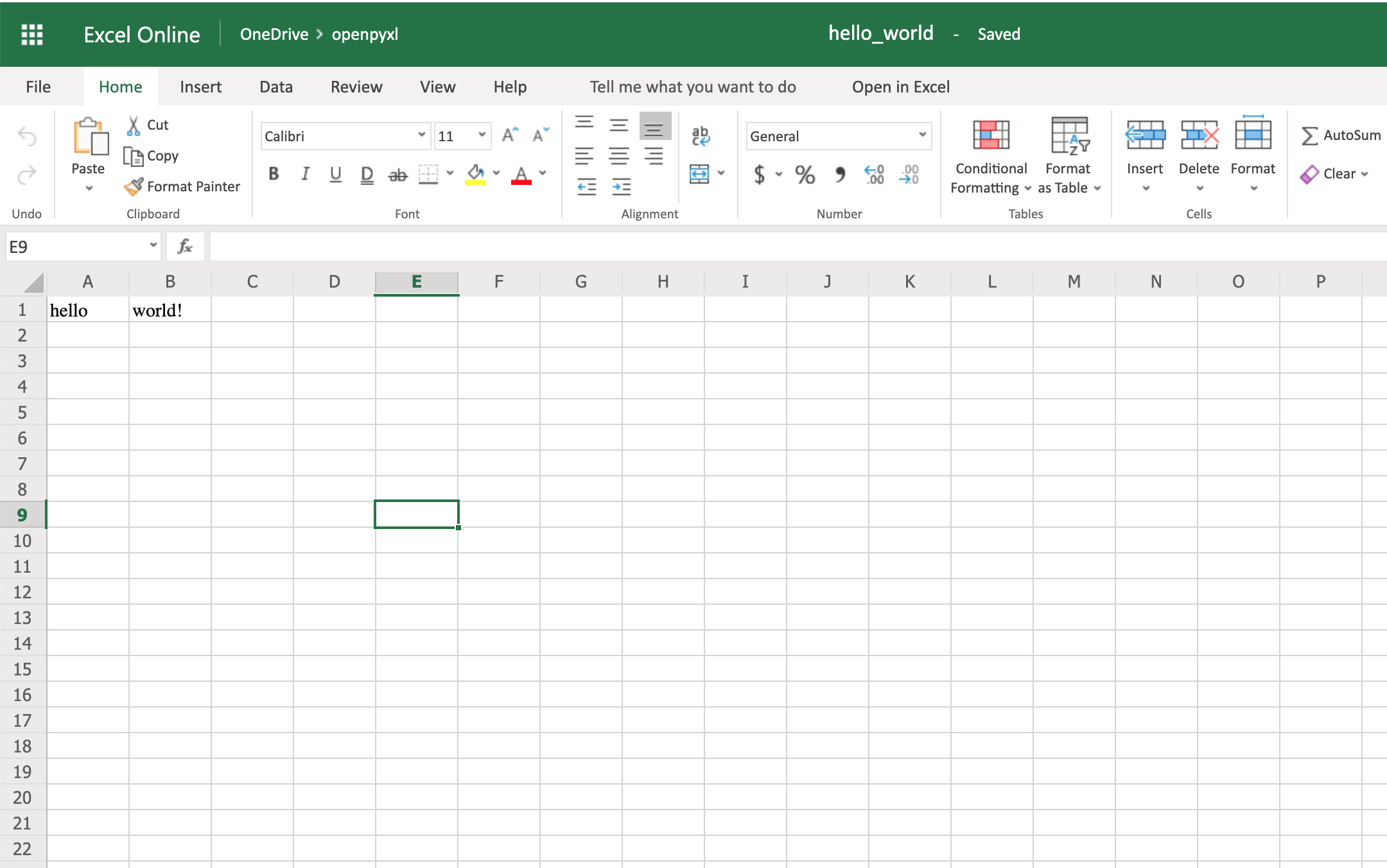
Woohoo, your first spreadsheet created!
Let’s start with the most essential thing one can do with a spreadsheet: read it.
You’ll go from a straightforward approach to reading a spreadsheet to more complex examples where you read the data and convert it into more useful Python structures.
Before you dive deep into some code examples, you should download this sample dataset and store it somewhere as sample.xlsx:
Download Dataset: Click here to download the dataset for the openpyxl exercise you'll be following in this tutorial.
This is one of the datasets you’ll be using throughout this tutorial, and it’s a spreadsheet with a sample of real data from Amazon’s online product reviews. This dataset is only a tiny fraction of what Amazon provides, but for testing purposes, it’s more than enough.
Finally, let’s start reading some spreadsheets! To begin with, open our sample spreadsheet:
>>> from openpyxl import load_workbook
>>> workbook = load_workbook(filename="sample.xlsx")
>>> workbook.sheetnames
['Sheet 1']

>>> sheet = workbook.active
>>> sheet
<Worksheet "Sheet 1">

>>> sheet.title
'Sheet 1'
In the code above, you first open the spreadsheet sample.xlsx using load_workbook(), and then you can use workbook.sheetnames to see all the sheets you have available to work with. After that, workbook.active selects the first available sheet and, in this case, you can see that it selects Sheet 1 automatically. Using these methods is the default way of opening a spreadsheet, and you’ll see it many times during this tutorial.
Now, after opening a spreadsheet, you can easily retrieve data from it like this:
>>> sheet["A1"]
<Cell 'Sheet 1'.A1>

>>> sheet["A1"].value
'marketplace'

>>> sheet["F10"].value
"G-Shock Men's Grey Sport Watch"
To return the actual value of a cell, you need to do .value. Otherwise, you’ll get the main Cell object. You can also use the method .cell() to retrieve a cell using index notation. Remember to add .value to get the actual value and not a Cell object:
>>> sheet.cell(row=10, column=6)
<Cell 'Sheet 1'.F10>

>>> sheet.cell(row=10, column=6).value
"G-Shock Men's Grey Sport Watch"
You can see that the results returned are the same, no matter which way you decide to go with. However, in this tutorial, you’ll be mostly using the first approach: ["A1"].
Note: Even though in Python you’re used to a zero-indexed notation, with spreadsheets you’ll always use a one-indexed notation where the first row or column always has index 1.
The above shows you the quickest way to open a spreadsheet. However, you can pass additional parameters to change the way a spreadsheet is loaded.
There are a few arguments you can pass to load_workbook() that change the way a spreadsheet is loaded. The most important ones are the following two Booleans:
Now that you’ve learned the basics about loading a spreadsheet, it’s about time you get to the fun part: the iteration and actual usage of the values within the spreadsheet.
This section is where you’ll learn all the different ways you can iterate through the data, but also how to convert that data into something usable and, more importantly, how to do it in a Pythonic way.
There are a few different ways you can iterate through the data depending on your needs.
You can slice the data with a combination of columns and rows:
>>> sheet["A1:C2"]
((<Cell 'Sheet 1'.A1>, <Cell 'Sheet 1'.B1>, <Cell 'Sheet 1'.C1>),
 (<Cell 'Sheet 1'.A2>, <Cell 'Sheet 1'.B2>, <Cell 'Sheet 1'.C2>))
You can get ranges of rows or columns:
>>> # Get all cells from column A
>>> sheet["A"]
(<Cell 'Sheet 1'.A1>,
 <Cell 'Sheet 1'.A2>,
 ...
 <Cell 'Sheet 1'.A99>,
 <Cell 'Sheet 1'.A100>)

>>> # Get all cells for a range of columns
>>> sheet["A:B"]
((<Cell 'Sheet 1'.A1>,
  <Cell 'Sheet 1'.A2>,
  ...
  <Cell 'Sheet 1'.A99>,
  <Cell 'Sheet 1'.A100>),
 (<Cell 'Sheet 1'.B1>,
  <Cell 'Sheet 1'.B2>,
  ...
  <Cell 'Sheet 1'.B99>,
  <Cell 'Sheet 1'.B100>))

>>> # Get all cells from row 5
>>> sheet[5]
(<Cell 'Sheet 1'.A5>,
 <Cell 'Sheet 1'.B5>,
 ...
 <Cell 'Sheet 1'.N5>,
 <Cell 'Sheet 1'.O5>)

>>> # Get all cells for a range of rows
>>> sheet[5:6]
((<Cell 'Sheet 1'.A5>,
  <Cell 'Sheet 1'.B5>,
  ...
  <Cell 'Sheet 1'.N5>,
  <Cell 'Sheet 1'.O5>),
 (<Cell 'Sheet 1'.A6>,
  <Cell 'Sheet 1'.B6>,
  ...
  <Cell 'Sheet 1'.N6>,
  <Cell 'Sheet 1'.O6>))
You’ll notice that all of the above examples return a tuple. If you want to refresh your memory on how to handle tuples in Python, check out the article on Lists and Tuples in Python.
There are also multiple ways of using normal Python generators to go through the data. The main methods you can use to achieve this are:
.iter_rows().iter_cols()Both methods can receive the following arguments:
min_rowmax_rowmin_colmax_colThese arguments are used to set boundaries for the iteration:
>>> for row in sheet.iter_rows(min_row=1,
...                            max_row=2,
...                            min_col=1,
...                            max_col=3):
...     print(row)
(<Cell 'Sheet 1'.A1>, <Cell 'Sheet 1'.B1>, <Cell 'Sheet 1'.C1>)
(<Cell 'Sheet 1'.A2>, <Cell 'Sheet 1'.B2>, <Cell 'Sheet 1'.C2>)


>>> for column in sheet.iter_cols(min_row=1,
...                               max_row=2,
...                               min_col=1,
...                               max_col=3):
...     print(column)
(<Cell 'Sheet 1'.A1>, <Cell 'Sheet 1'.A2>)
(<Cell 'Sheet 1'.B1>, <Cell 'Sheet 1'.B2>)
(<Cell 'Sheet 1'.C1>, <Cell 'Sheet 1'.C2>)
You’ll notice that in the first example, when iterating through the rows using .iter_rows(), you get one tuple element per row selected. While when using .iter_cols() and iterating through columns, you’ll get one tuple per column instead.
One additional argument you can pass to both methods is the Boolean values_only. When it’s set to True, the values of the cell are returned, instead of the Cell object:
>>> for value in sheet.iter_rows(min_row=1,
...                              max_row=2,
...                              min_col=1,
...                              max_col=3,
...                              values_only=True):
...     print(value)
('marketplace', 'customer_id', 'review_id')
('US', 3653882, 'R3O9SGZBVQBV76')
If you want to iterate through the whole dataset, then you can also use the attributes .rows or .columns directly, which are shortcuts to using .iter_rows() and .iter_cols() without any arguments:
>>> for row in sheet.rows:
...     print(row)
(<Cell 'Sheet 1'.A1>, <Cell 'Sheet 1'.B1>, <Cell 'Sheet 1'.C1>
...
<Cell 'Sheet 1'.M100>, <Cell 'Sheet 1'.N100>, <Cell 'Sheet 1'.O100>)
These shortcuts are very useful when you’re iterating through the whole dataset.
Now that you know the basics of iterating through the data in a workbook, let’s look at smart ways of converting that data into Python structures.
As you saw earlier, the result from all iterations comes in the form of tuples. However, since a tuple is nothing more than an immutable list, you can easily access its data and transform it into other structures.
For example, say you want to extract product information from the sample.xlsx spreadsheet and into a dictionary where each key is a product ID.
A straightforward way to do this is to iterate over all the rows, pick the columns you know are related to product information, and then store that in a dictionary. Let’s code this out!
First of all, have a look at the headers and see what information you care most about:
>>> for value in sheet.iter_rows(min_row=1,
...                              max_row=1,
...                              values_only=True):
...     print(value)
('marketplace', 'customer_id', 'review_id', 'product_id', ...)
This code returns a list of all the column names you have in the spreadsheet. To start, grab the columns with names:
product_idproduct_parentproduct_titleproduct_categoryLucky for you, the columns you need are all next to each other so you can use the min_column and max_column to easily get the data you want:
>>> for value in sheet.iter_rows(min_row=2,
...                              min_col=4,
...                              max_col=7,
...                              values_only=True):
...     print(value)
('B00FALQ1ZC', 937001370, 'Invicta Women\'s 15150 "Angel" 18k Yellow...)
('B00D3RGO20', 484010722, "Kenneth Cole New York Women's KC4944...)
...
Nice! Now that you know how to get all the important product information you need, let’s put that data into a dictionary:
import json
from openpyxl import load_workbook

workbook = load_workbook(filename="sample.xlsx")
sheet = workbook.active

products = {}

# Using the values_only because you want to return the cells' values
for row in sheet.iter_rows(min_row=2,
                           min_col=4,
                           max_col=7,
                           values_only=True):
    product_id = row[0]
    product = {
        "parent": row[1],
        "title": row[2],
        "category": row[3]
    }
    products[product_id] = product

# Using json here to be able to format the output for displaying later
print(json.dumps(products))
The code above returns a JSON similar to this:
{
  "B00FALQ1ZC": {
    "parent": 937001370,
    "title": "Invicta Women's 15150 ...",
    "category": "Watches"
  },
  "B00D3RGO20": {
    "parent": 484010722,
    "title": "Kenneth Cole New York ...",
    "category": "Watches"
  }
}
Here you can see that the output is trimmed to 2 products only, but if you run the script as it is, then you should get 98 products.
To finalize the reading section of this tutorial, let’s dive into Python classes and see how you could improve on the example above and better structure the data.
For this, you’ll be using the new Python Data Classes that are available from Python 3.7. If you’re using an older version of Python, then you can use the default Classes instead.
So, first things first, let’s look at the data you have and decide what you want to store and how you want to store it.
As you saw right at the start, this data comes from Amazon, and it’s a list of product reviews. You can check the list of all the columns and their meaning on Amazon.
There are two significant elements you can extract from the data available:
A Product has:
The Review has a few more fields:
You can ignore a few of the review fields to make things a bit simpler.
So, a straightforward implementation of these two classes could be written in a separate file classes.py:
import datetime
from dataclasses import dataclass

@dataclass
class Product:
    id: str
    parent: str
    title: str
    category: str

@dataclass
class Review:
    id: str
    customer_id: str
    stars: int
    headline: str
    body: str
    date: datetime.datetime
After defining your data classes, you need to convert the data from the spreadsheet into these new structures.
Before doing the conversion, it’s worth looking at our header again and creating a mapping between columns and the fields you need:
>>> for value in sheet.iter_rows(min_row=1,
...                              max_row=1,
...                              values_only=True):
...     print(value)
('marketplace', 'customer_id', 'review_id', 'product_id', ...)

>>> # Or an alternative
>>> for cell in sheet[1]:
...     print(cell.value)
marketplace
customer_id
review_id
product_id
product_parent
...
Let’s create a file mapping.py where you have a list of all the field names and their column location (zero-indexed) on the spreadsheet:
# Product fields
PRODUCT_ID = 3
PRODUCT_PARENT = 4
PRODUCT_TITLE = 5
PRODUCT_CATEGORY = 6

# Review fields
REVIEW_ID = 2
REVIEW_CUSTOMER = 1
REVIEW_STARS = 7
REVIEW_HEADLINE = 12
REVIEW_BODY = 13
REVIEW_DATE = 14
You don’t necessarily have to do the mapping above. It’s more for readability when parsing the row data, so you don’t end up with a lot of magic numbers lying around.
Finally, let’s look at the code needed to parse the spreadsheet data into a list of product and review objects:
from datetime import datetime
from openpyxl import load_workbook
from classes import Product, Review
from mapping import PRODUCT_ID, PRODUCT_PARENT, PRODUCT_TITLE, \
    PRODUCT_CATEGORY, REVIEW_DATE, REVIEW_ID, REVIEW_CUSTOMER, \
    REVIEW_STARS, REVIEW_HEADLINE, REVIEW_BODY

# Using the read_only method since you're not gonna be editing the spreadsheet
workbook = load_workbook(filename="sample.xlsx", read_only=True)
sheet = workbook.active

products = []
reviews = []

# Using the values_only because you just want to return the cell value
for row in sheet.iter_rows(min_row=2, values_only=True):
    product = Product(id=row[PRODUCT_ID],
                      parent=row[PRODUCT_PARENT],
                      title=row[PRODUCT_TITLE],
                      category=row[PRODUCT_CATEGORY])
    products.append(product)

    # You need to parse the date from the spreadsheet into a datetime format
    spread_date = row[REVIEW_DATE]
    parsed_date = datetime.strptime(spread_date, "%Y-%m-%d")

    review = Review(id=row[REVIEW_ID],
                    customer_id=row[REVIEW_CUSTOMER],
                    stars=row[REVIEW_STARS],
                    headline=row[REVIEW_HEADLINE],
                    body=row[REVIEW_BODY],
                    date=parsed_date)
    reviews.append(review)

print(products[0])
print(reviews[0])
After you run the code above, you should get some output like this:
Product(id='B00FALQ1ZC', parent=937001370, ...)
Review(id='R3O9SGZBVQBV76', customer_id=3653882, ...)
That’s it! Now you should have the data in a very simple and digestible class format, and you can start thinking of storing this in a Database or any other type of data storage you like.
Using this kind of OOP strategy to parse spreadsheets makes handling the data much simpler later on.
Before you start creating very complex spreadsheets, have a quick look at an example of how to append data to an existing spreadsheet.
Go back to the first example spreadsheet you created (hello_world.xlsx) and try opening it and appending some data to it, like this:
from openpyxl import load_workbook

# Start by opening the spreadsheet and selecting the main sheet
workbook = load_workbook(filename="hello_world.xlsx")
sheet = workbook.active

# Write what you want into a specific cell
sheet["C1"] = "writing ;)"

# Save the spreadsheet
workbook.save(filename="hello_world_append.xlsx"
Et voilà, if you open the new hello_world_append.xlsx spreadsheet, you’ll see the following change:
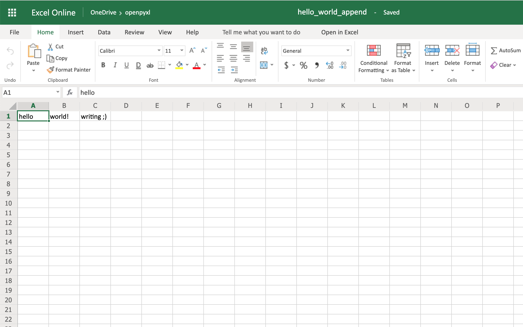
Notice the additional writing ;) on cell C1.
There are a lot of different things you can write to a spreadsheet, from simple text or number values to complex formulas, charts, or even images.
Let’s start creating some spreadsheets!
Previously, you saw a very quick example of how to write “Hello world!” into a spreadsheet, so you can start with that:
 1 from openpyxl import Workbook
 2
 3 filename = "hello_world.xlsx"
 4
 5 workbook = Workbook()
 6 sheet = workbook.active
 7
 8 sheet["A1"] = "hello"
 9 sheet["B1"] = "world!"
10
11 workbook.save(filename=filename)
The highlighted lines in the code above are the most important ones for writing. In the code, you can see that:
Even though these lines above can be straightforward, it’s still good to know them well for when things get a bit more complicated.
Note: You’ll be using the hello_world.xlsx spreadsheet for some of the upcoming examples, so keep it handy.
One thing you can do to help with coming code examples is add the following method to your Python file or console:
>>> def print_rows():
...     for row in sheet.iter_rows(values_only=True):
...         print(row)
It makes it easier to print all of your spreadsheet values by just calling print_rows().
Before you get into the more advanced topics, it’s good for you to know how to manage the most simple elements of a spreadsheet.
You already learned how to add values to a spreadsheet like this:
>>> sheet["A1"] = "value"
There’s another way you can do this, by first selecting a cell and then changing its value:
>>> cell = sheet["A1"]
>>> cell
<Cell 'Sheet'.A1>

>>> cell.value
'hello'

>>> cell.value = "hey"
>>> cell.value
'hey'
The new value is only stored into the spreadsheet once you call workbook.save().
The openpyxl creates a cell when adding a value, if that cell didn’t exist before:
>>> # Before, our spreadsheet has only 1 row
>>> print_rows()
('hello', 'world!')

>>> # Try adding a value to row 10
>>> sheet["B10"] = "test"
>>> print_rows()
('hello', 'world!')
(None, None)
(None, None)
(None, None)
(None, None)
(None, None)
(None, None)
(None, None)
(None, None)
(None, 'test')
As you can see, when trying to add a value to cell B10, you end up with a tuple with 10 rows, just so you can have that test value.
One of the most common things you have to do when manipulating spreadsheets is adding or removing rows and columns. The openpyxl package allows you to do that in a very straightforward way by using the methods:
.insert_rows().delete_rows().insert_cols().delete_cols()Every single one of those methods can receive two arguments:
idxamountUsing our basic hello_world.xlsx example again, let’s see how these methods work:
>>> print_rows()
('hello', 'world!')

>>> # Insert a column before the existing column 1 ("A")
>>> sheet.insert_cols(idx=1)
>>> print_rows()
(None, 'hello', 'world!')

>>> # Insert 5 columns between column 2 ("B") and 3 ("C")
>>> sheet.insert_cols(idx=3, amount=5)
>>> print_rows()
(None, 'hello', None, None, None, None, None, 'world!')

>>> # Delete the created columns
>>> sheet.delete_cols(idx=3, amount=5)
>>> sheet.delete_cols(idx=1)
>>> print_rows()
('hello', 'world!')

>>> # Insert a new row in the beginning
>>> sheet.insert_rows(idx=1)
>>> print_rows()
(None, None)
('hello', 'world!')

>>> # Insert 3 new rows in the beginning
>>> sheet.insert_rows(idx=1, amount=3)
>>> print_rows()
(None, None)
(None, None)
(None, None)
(None, None)
('hello', 'world!')

>>> # Delete the first 4 rows
>>> sheet.delete_rows(idx=1, amount=4)
>>> print_rows()
('hello', 'world!')
The only thing you need to remember is that when inserting new data (rows or columns), the insertion happens before the idx parameter.
So, if you do insert_rows(1), it inserts a new row before the existing first row.
It’s the same for columns: when you call insert_cols(2), it inserts a new column right before the already existing second column (B).
However, when deleting rows or columns, .delete_... deletes data starting from the index passed as an argument.
For example, when doing delete_rows(2) it deletes row 2, and when doing delete_cols(3) it deletes the third column (C).
Sheet management is also one of those things you might need to know, even though it might be something that you don’t use that often.
If you look back at the code examples from this tutorial, you’ll notice the following recurring piece of code:
sheet = workbook.active
This is the way to select the default sheet from a spreadsheet. However, if you’re opening a spreadsheet with multiple sheets, then you can always select a specific one like this:
>>> # Let's say you have two sheets: "Products" and "Company Sales"
>>> workbook.sheetnames
['Products', 'Company Sales']

>>> # You can select a sheet using its title
>>> products_sheet = workbook["Products"]
>>> sales_sheet = workbook["Company Sales"]
You can also change a sheet title very easily:
>>> workbook.sheetnames
['Products', 'Company Sales']

>>> products_sheet = workbook["Products"]
>>> products_sheet.title = "New Products"

>>> workbook.sheetnames
['New Products', 'Company Sales']
If you want to create or delete sheets, then you can also do that with .create_sheet() and .remove():
>>> workbook.sheetnames
['Products', 'Company Sales']

>>> operations_sheet = workbook.create_sheet("Operations")
>>> workbook.sheetnames
['Products', 'Company Sales', 'Operations']

>>> # You can also define the position to create the sheet at
>>> hr_sheet = workbook.create_sheet("HR", 0)
>>> workbook.sheetnames
['HR', 'Products', 'Company Sales', 'Operations']

>>> # To remove them, just pass the sheet as an argument to the .remove()
>>> workbook.remove(operations_sheet)
>>> workbook.sheetnames
['HR', 'Products', 'Company Sales']

>>> workbook.remove(hr_sheet)
>>> workbook.sheetnames
['Products', 'Company Sales']
One other thing you can do is make duplicates of a sheet using copy_worksheet():
>>> workbook.sheetnames
['Products', 'Company Sales']

>>> products_sheet = workbook["Products"]
>>> workbook.copy_worksheet(products_sheet)
<Worksheet "Products Copy">

>>> workbook.sheetnames
['Products', 'Company Sales', 'Products Copy']
If you open your spreadsheet after saving the above code, you’ll notice that the sheet Products Copy is a duplicate of the sheet Products.
Something that you might want to do when working with big spreadsheets is to freeze a few rows or columns, so they remain visible when you scroll right or down.
Freezing data allows you to keep an eye on important rows or columns, regardless of where you scroll in the spreadsheet.
Again, openpyxl also has a way to accomplish this by using the worksheet freeze_panes attribute. For this example, go back to our sample.xlsx spreadsheet and try doing the following:
>>> workbook = load_workbook(filename="sample.xlsx")
>>> sheet = workbook.active
>>> sheet.freeze_panes = "C2"
>>> workbook.save("sample_frozen.xlsx")
If you open the sample_frozen.xlsx spreadsheet in your favorite spreadsheet editor, you’ll notice that row 1 and columns A and B are frozen and are always visible no matter where you navigate within the spreadsheet.
This feature is handy, for example, to keep headers within sight, so you always know what each column represents.
Here’s how it looks in the editor:
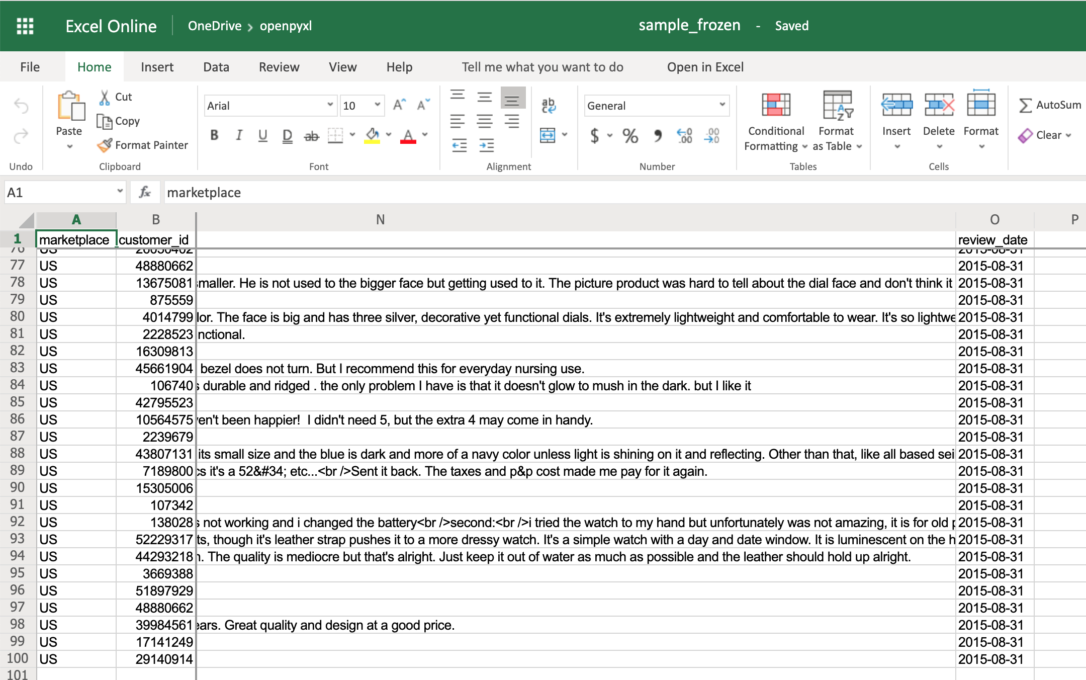
Notice how you’re at the end of the spreadsheet, and yet, you can see both row 1 and columns A and B.
You can use openpyxl to add filters and sorts to your spreadsheet. However, when you open the spreadsheet, the data won’t be rearranged according to these sorts and filters.
At first, this might seem like a pretty useless feature, but when you’re programmatically creating a spreadsheet that is going to be sent and used by somebody else, it’s still nice to at least create the filters and allow people to use it afterward.
The code below is an example of how you would add some filters to our existing sample.xlsx spreadsheet:
>>> # Check the used spreadsheet space using the attribute "dimensions"
>>> sheet.dimensions
'A1:O100'

>>> sheet.auto_filter.ref = "A1:O100"
>>> workbook.save(filename="sample_with_filters.xlsx")
You should now see the filters created when opening the spreadsheet in your editor:
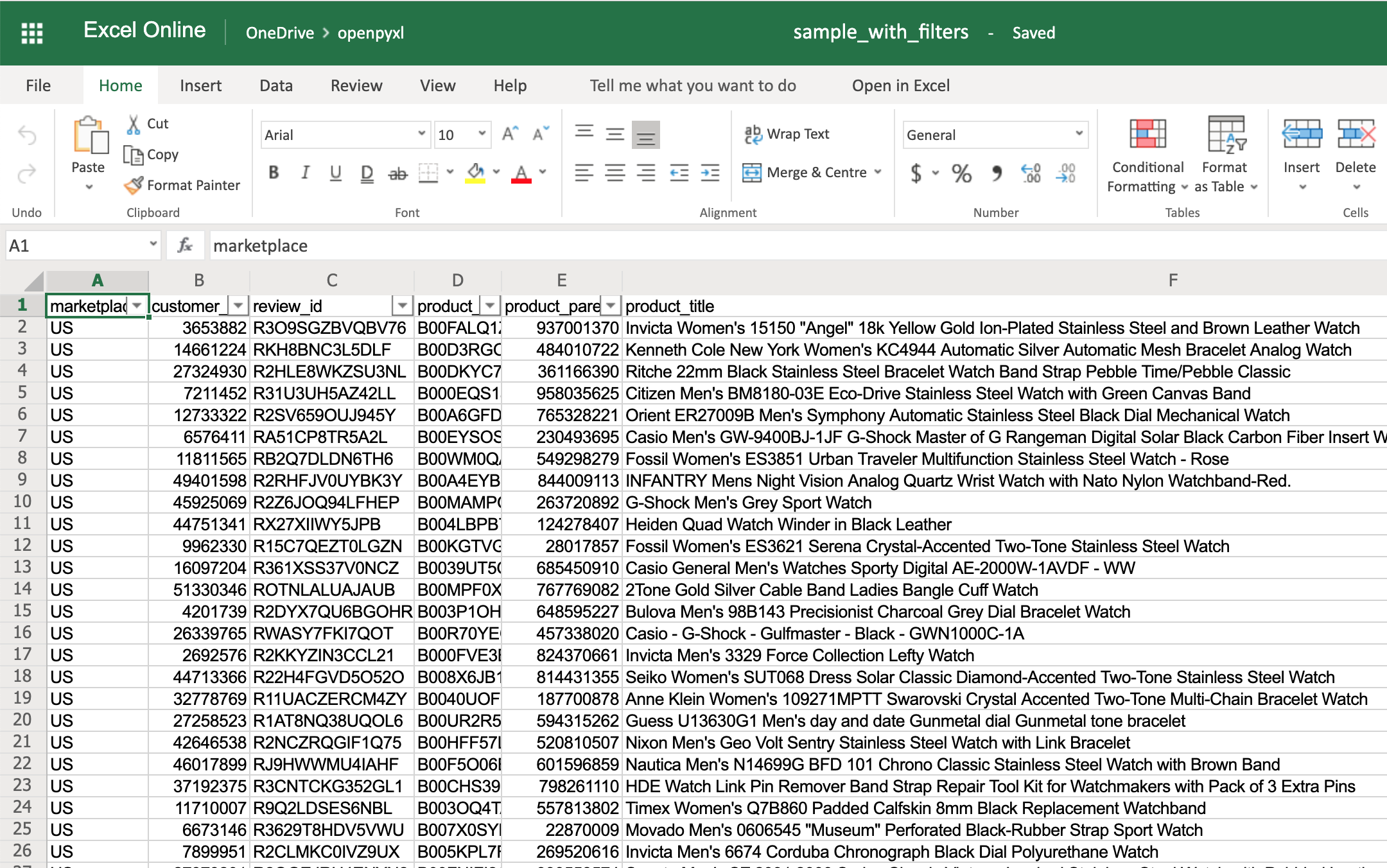
You don’t have to use sheet.dimensions if you know precisely which part of the spreadsheet you want to apply filters to.
Formulas (or formulae) are one of the most powerful features of spreadsheets.
They gives you the power to apply specific mathematical equations to a range of cells. Using formulas with openpyxl is as simple as editing the value of a cell.
You can see the list of formulas supported by openpyxl:
>>> from openpyxl.utils import FORMULAE
>>> FORMULAE
frozenset({'ABS',
           'ACCRINT',
           'ACCRINTM',
           'ACOS',
           'ACOSH',
           'AMORDEGRC',
           'AMORLINC',
           'AND',
           ...
           'YEARFRAC',
           'YIELD',
           'YIELDDISC',
           'YIELDMAT',
           'ZTEST'})
Let’s add some formulas to our sample.xlsx spreadsheet.
Starting with something easy, let’s check the average star rating for the 99 reviews within the spreadsheet:
>>> # Star rating is column "H"
>>> sheet["P2"] = "=AVERAGE(H2:H100)"
>>> workbook.save(filename="sample_formulas.xlsx")
If you open the spreadsheet now and go to cell P2, you should see that its value is: 4.18181818181818. Have a look in the editor:
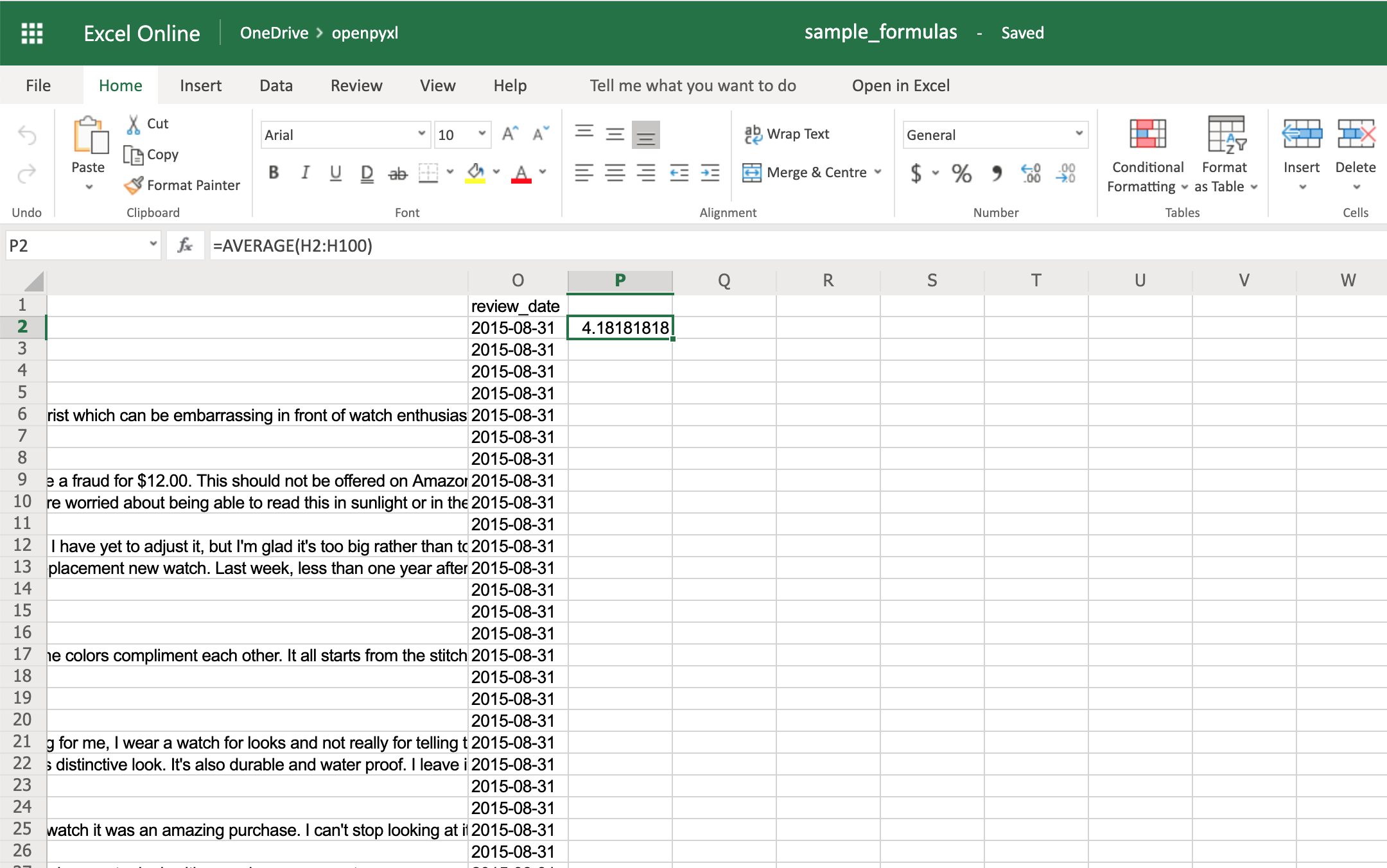
You can use the same methodology to add any formulas to your spreadsheet. For example, let’s count the number of reviews that had helpful votes:
>>> # The helpful votes are counted on column "I"
>>> sheet["P3"] = '=COUNTIF(I2:I100, ">0")'
>>> workbook.save(filename="sample_formulas.xlsx")
You should get the number 21 on your P3 spreadsheet cell like so:
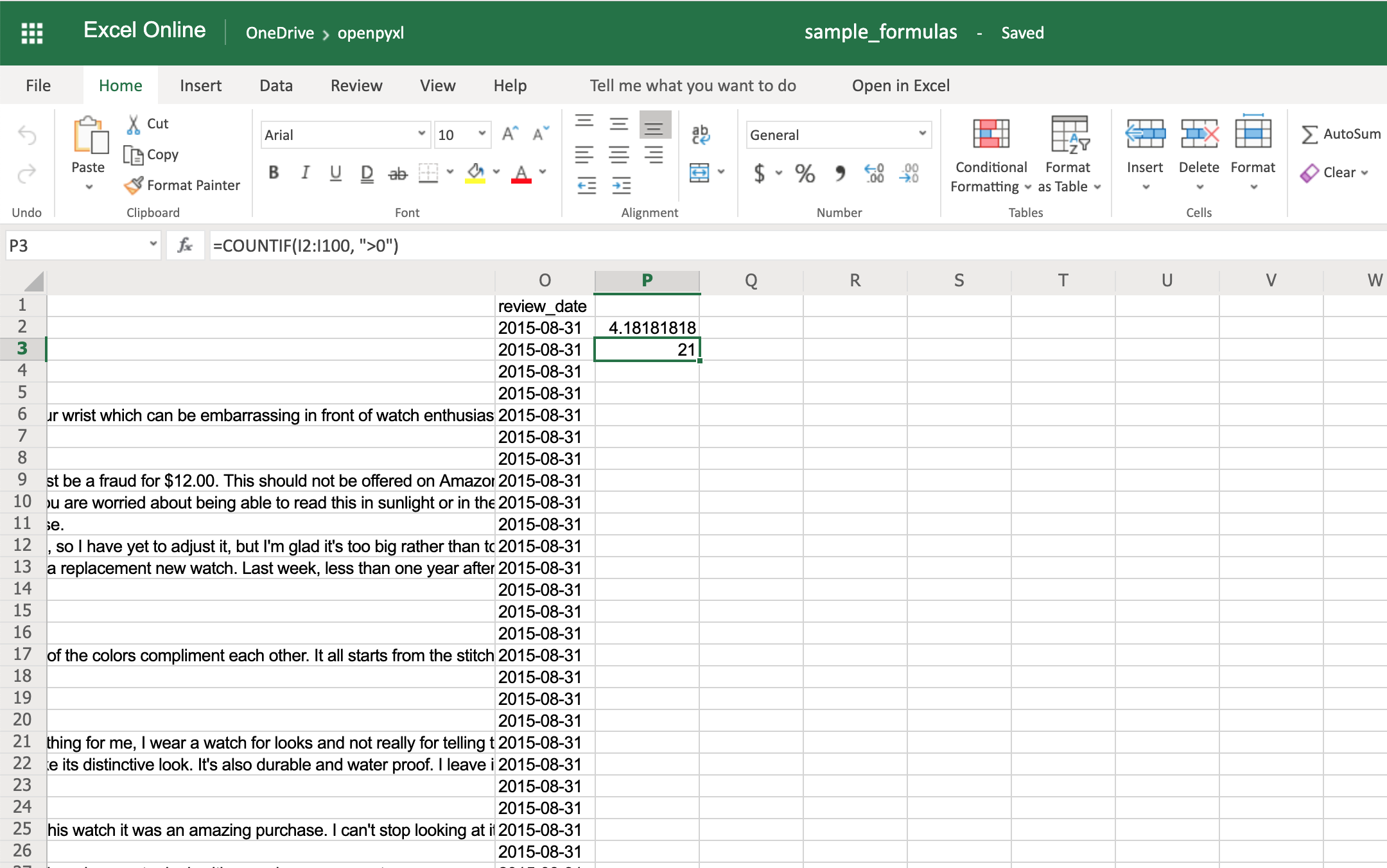
You’ll have to make sure that the strings within a formula are always in double quotes, so you either have to use single quotes around the formula like in the example above or you’ll have to escape the double quotes inside the formula: "=COUNTIF(I2:I100, \">0\")".
There are a ton of other formulas you can add to your spreadsheet using the same procedure you tried above. Give it a go yourself!
Even though styling a spreadsheet might not be something you would do every day, it’s still good to know how to do it.
Using openpyxl, you can apply multiple styling options to your spreadsheet, including fonts, borders, colors, and so on. Have a look at the openpyxl documentation to learn more.
You can also choose to either apply a style directly to a cell or create a template and reuse it to apply styles to multiple cells.
Let’s start by having a look at simple cell styling, using our sample.xlsx again as the base spreadsheet:
>>> # Import necessary style classes
>>> from openpyxl.styles import Font, Color, Alignment, Border, Side, colors

>>> # Create a few styles
>>> bold_font = Font(bold=True)
>>> big_red_text = Font(color=colors.RED, size=20)
>>> center_aligned_text = Alignment(horizontal="center")
>>> double_border_side = Side(border_style="double")
>>> square_border = Border(top=double_border_side,
...                        right=double_border_side,
...                        bottom=double_border_side,
...                        left=double_border_side)

>>> # Style some cells!
>>> sheet["A2"].font = bold_font
>>> sheet["A3"].font = big_red_text
>>> sheet["A4"].alignment = center_aligned_text
>>> sheet["A5"].border = square_border
>>> workbook.save(filename="sample_styles.xlsx")
If you open your spreadsheet now, you should see quite a few different styles on the first 5 cells of column A:
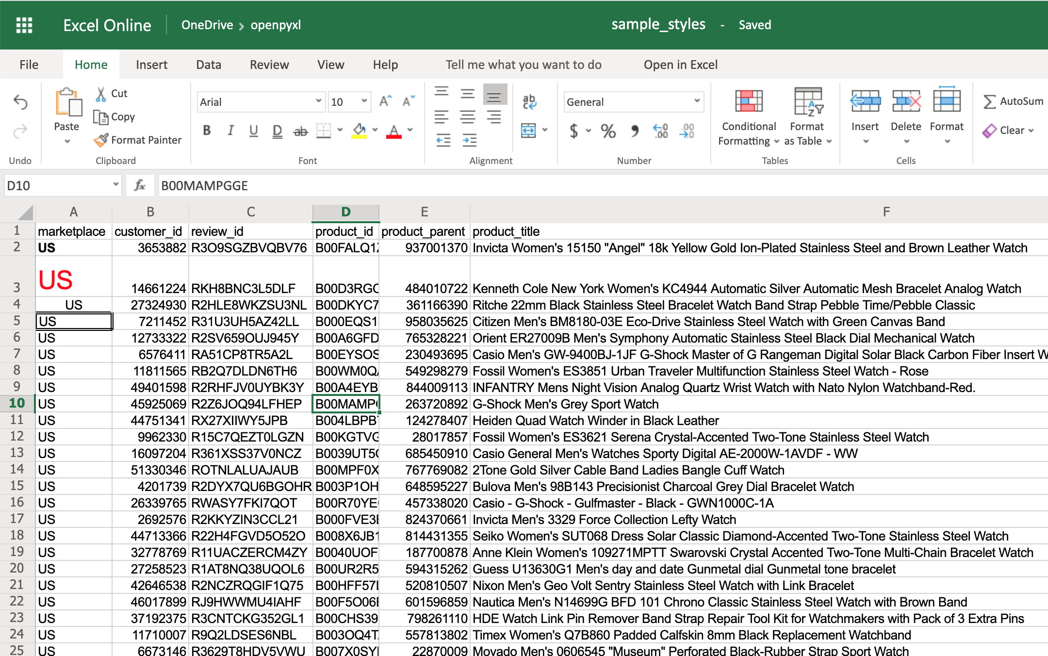
There you go. You got:
Note: For the colors, you can also use HEX codes instead by doing Font(color="C70E0F").
You can also combine styles by simply adding them to the cell at the same time:
>>> # Reusing the same styles from the example above
>>> sheet["A6"].alignment = center_aligned_text
>>> sheet["A6"].font = big_red_text
>>> sheet["A6"].border = square_border
>>> workbook.save(filename="sample_styles.xlsx")
Have a look at cell A6 here:
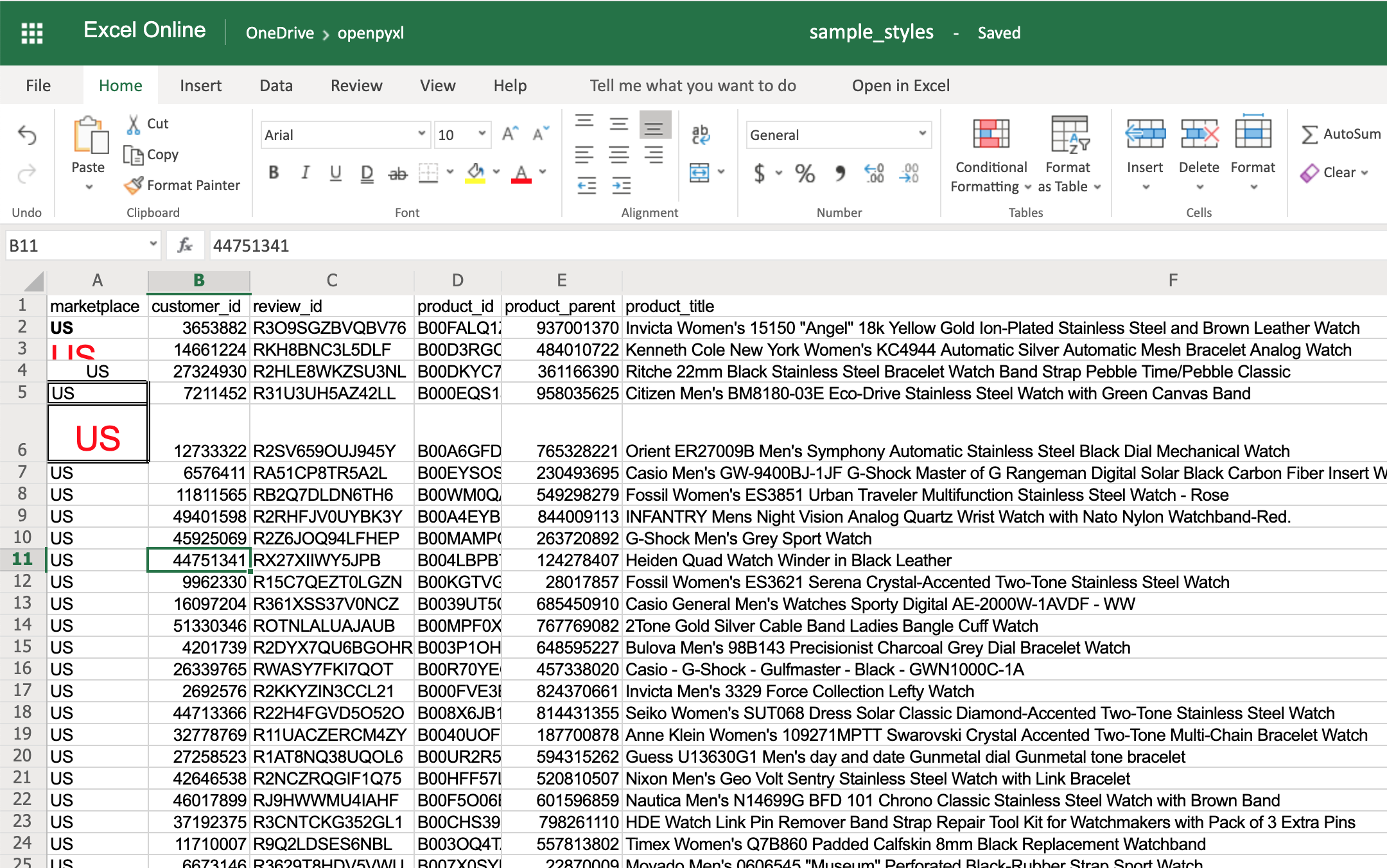
When you want to apply multiple styles to one or several cells, you can use a NamedStyle class instead, which is like a style template that you can use over and over again. Have a look at the example below:
>>> from openpyxl.styles import NamedStyle

>>> # Let's create a style template for the header row
>>> header = NamedStyle(name="header")
>>> header.font = Font(bold=True)
>>> header.border = Border(bottom=Side(border_style="thin"))
>>> header.alignment = Alignment(horizontal="center", vertical="center")

>>> # Now let's apply this to all first row (header) cells
>>> header_row = sheet[1]
>>> for cell in header_row:
...     cell.style = header

>>> workbook.save(filename="sample_styles.xlsx")
If you open the spreadsheet now, you should see that its first row is bold, the text is aligned to the center, and there’s a small bottom border! Have a look below:
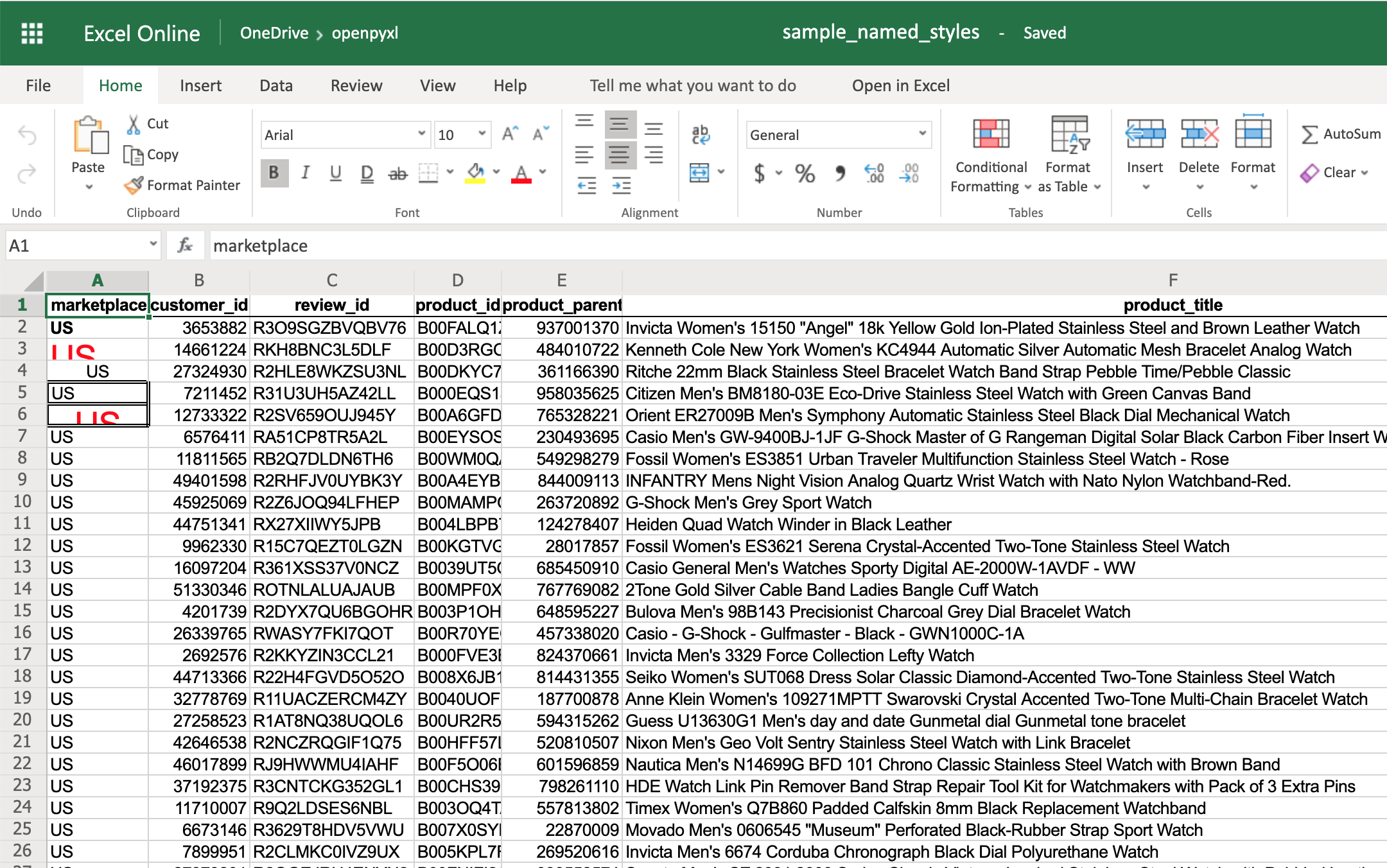
As you saw above, there are many options when it comes to styling, and it depends on the use case, so feel free to check openpyxl documentation and see what other things you can do.
This feature is one of my personal favorites when it comes to adding styles to a spreadsheet.
It’s a much more powerful approach to styling because it dynamically applies styles according to how the data in the spreadsheet changes.
In a nutshell, conditional formatting allows you to specify a list of styles to apply to a cell (or cell range) according to specific conditions.
For example, a widespread use case is to have a balance sheet where all the negative totals are in red, and the positive ones are in green. This formatting makes it much more efficient to spot good vs bad periods.
Without further ado, let’s pick our favorite spreadsheet—sample.xlsx—and add some conditional formatting.
You can start by adding a simple one that adds a red background to all reviews with less than 3 stars:
>>> from openpyxl.styles import PatternFill, colors
>>> from openpyxl.styles.differential import DifferentialStyle
>>> from openpyxl.formatting.rule import Rule

>>> red_background = PatternFill(bgColor=colors.RED)
>>> diff_style = DifferentialStyle(fill=red_background)
>>> rule = Rule(type="expression", dxf=diff_style)
>>> rule.formula = ["$H1<3"]
>>> sheet.conditional_formatting.add("A1:O100", rule)
>>> workbook.save("sample_conditional_formatting.xlsx")
Now you’ll see all the reviews with a star rating below 3 marked with a red background:
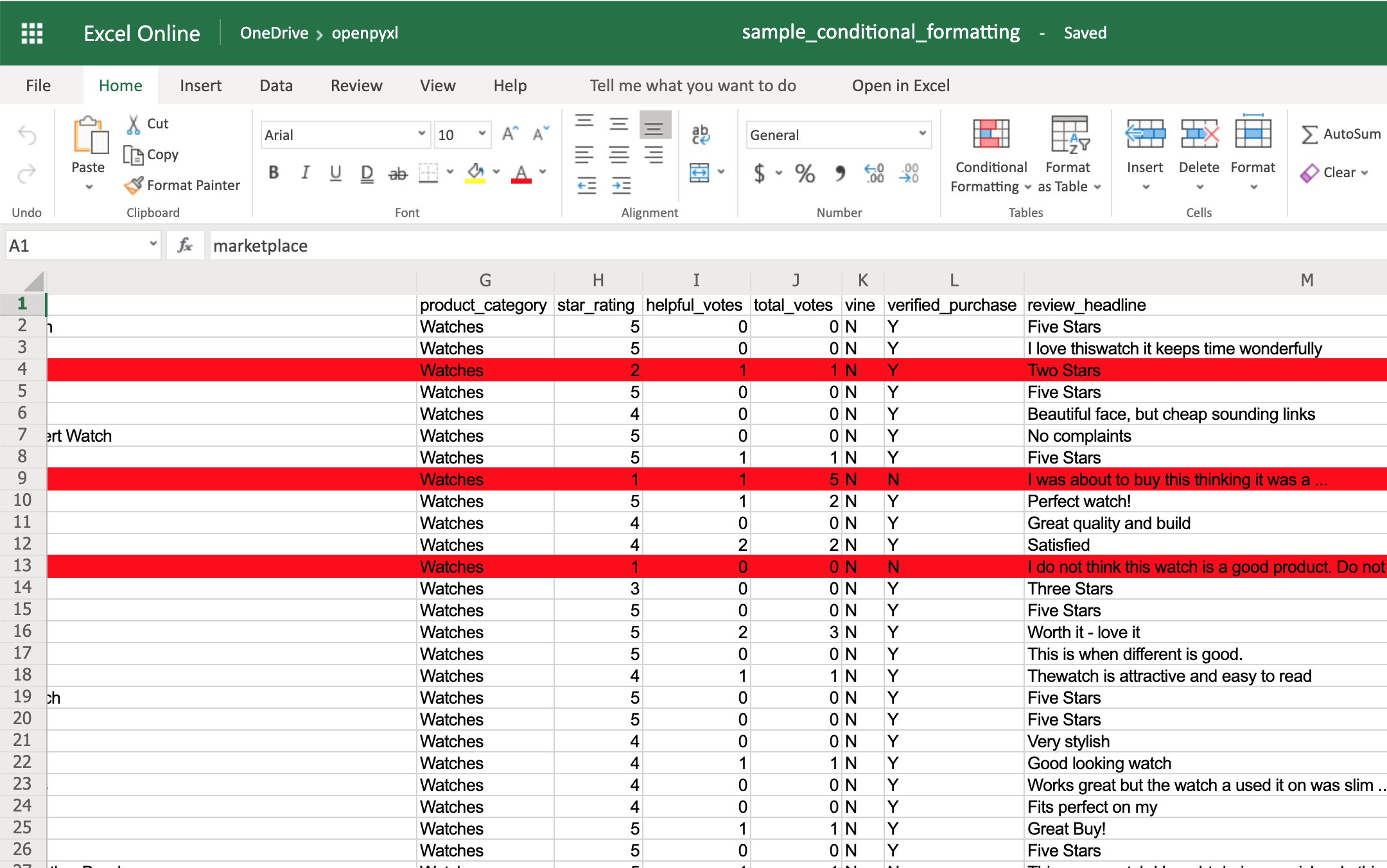
Code-wise, the only things that are new here are the objects DifferentialStyle and Rule:
DifferentialStyle is quite similar to NamedStyle, which you already saw above, and it’s used to aggregate multiple styles such as fonts, borders, alignment, and so forth.Rule is responsible for selecting the cells and applying the styles if the cells match the rule’s logic.Using a Rule object, you can create numerous conditional formatting scenarios.
However, for simplicity sake, the openpyxl package offers 3 built-in formats that make it easier to create a few common conditional formatting patterns. These built-ins are:
ColorScaleIconSetDataBarThe ColorScale gives you the ability to create color gradients:
>>> from openpyxl.formatting.rule import ColorScaleRule
>>> color_scale_rule = ColorScaleRule(start_type="min",
...                                   start_color=colors.RED,
...                                   end_type="max",
...                                   end_color=colors.GREEN)

>>> # Again, let's add this gradient to the star ratings, column "H"
>>> sheet.conditional_formatting.add("H2:H100", color_scale_rule)
>>> workbook.save(filename="sample_conditional_formatting_color_scale.xlsx")
Now you should see a color gradient on column H, from red to green, according to the star rating:
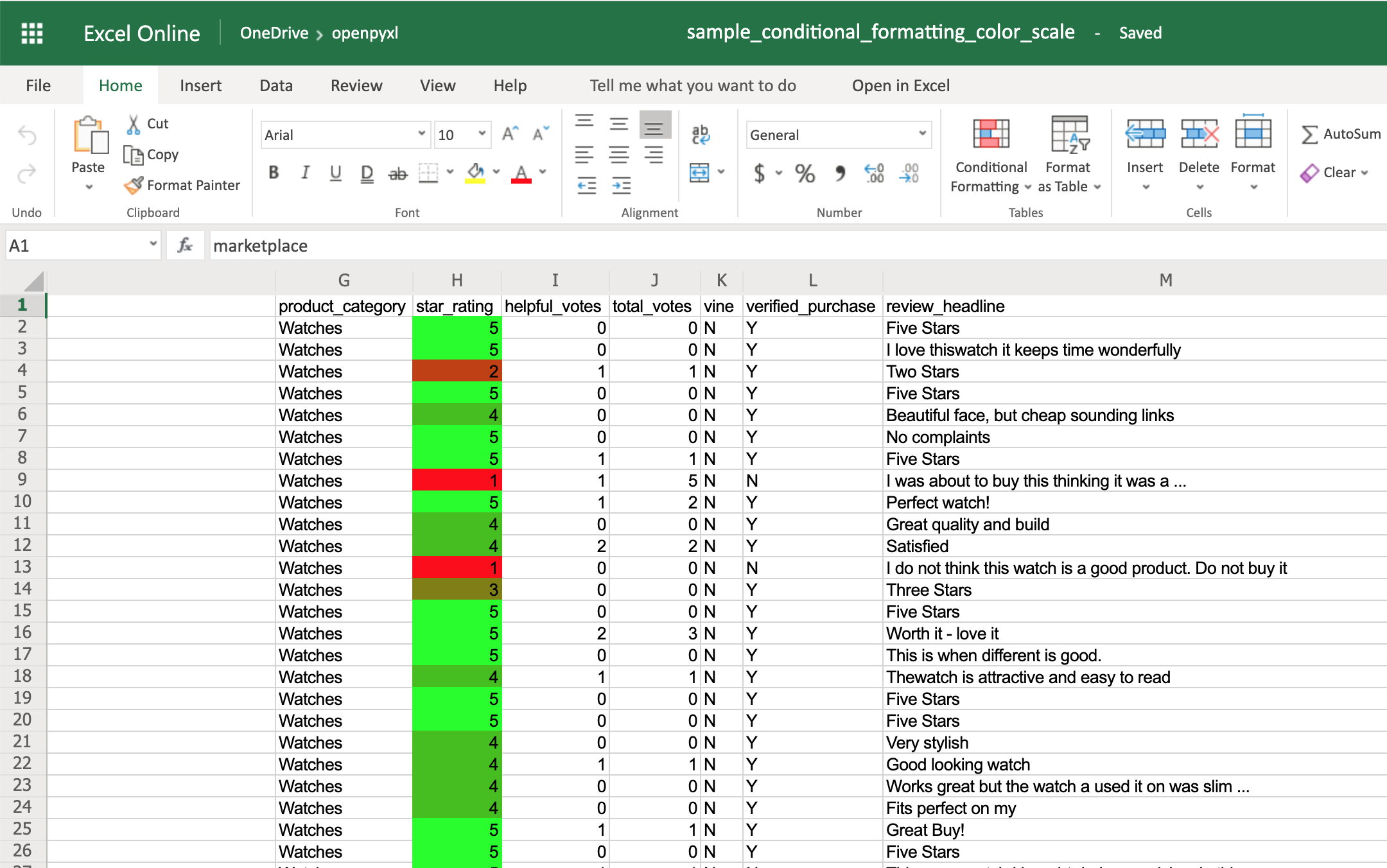
You can also add a third color and make two gradients instead:
>>> from openpyxl.formatting.rule import ColorScaleRule
>>> color_scale_rule = ColorScaleRule(start_type="num",
...                                   start_value=1,
...                                   start_color=colors.RED,
...                                   mid_type="num",
...                                   mid_value=3,
...                                   mid_color=colors.YELLOW,
...                                   end_type="num",
...                                   end_value=5,
...                                   end_color=colors.GREEN)

>>> # Again, let's add this gradient to the star ratings, column "H"
>>> sheet.conditional_formatting.add("H2:H100", color_scale_rule)
>>> workbook.save(filename="sample_conditional_formatting_color_scale_3.xlsx")
This time, you’ll notice that star ratings between 1 and 3 have a gradient from red to yellow, and star ratings between 3 and 5 have a gradient from yellow to green:
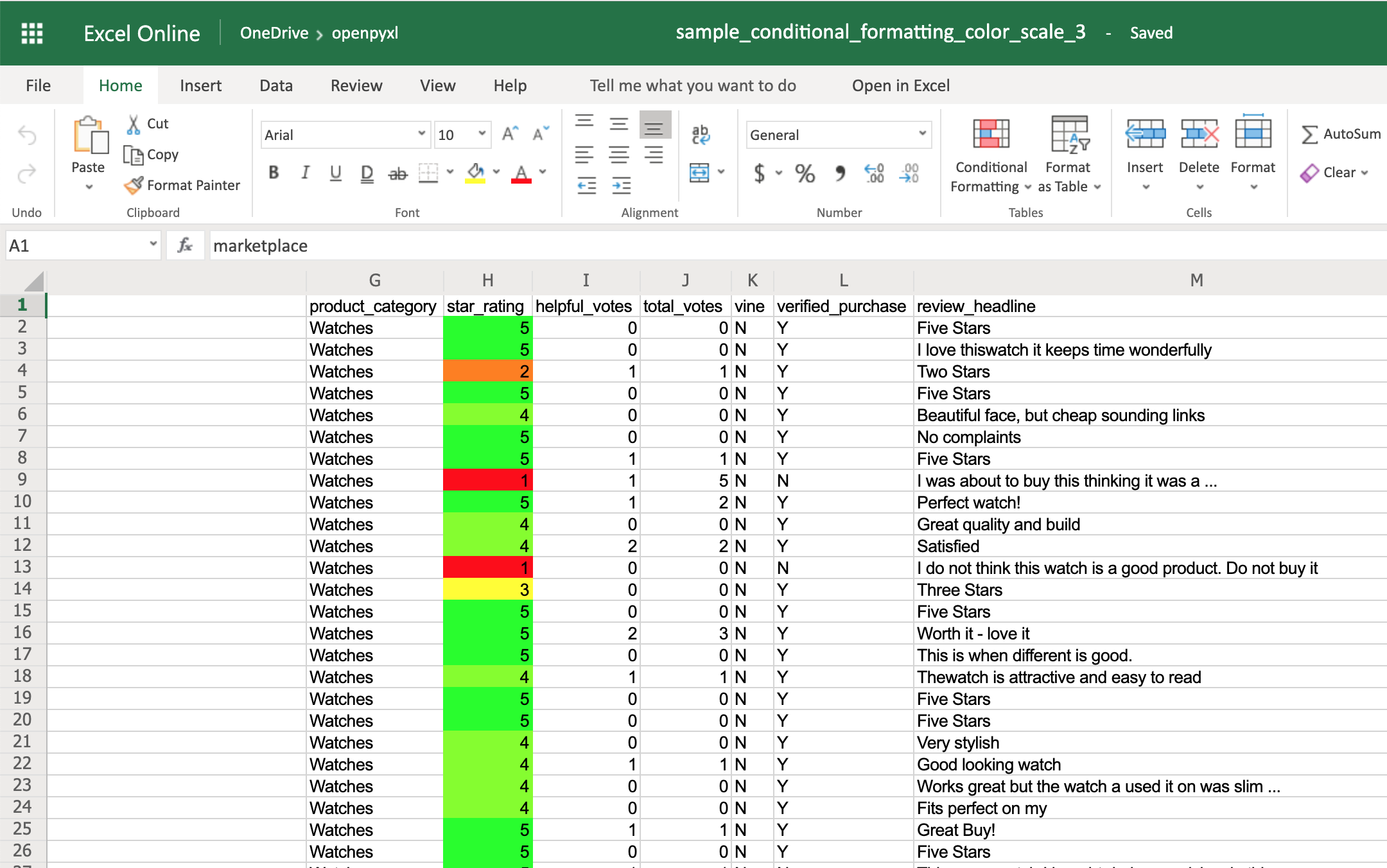
The IconSet allows you to add an icon to the cell according to its value:
>>> from openpyxl.formatting.rule import IconSetRule

>>> icon_set_rule = IconSetRule("5Arrows", "num", [1, 2, 3, 4, 5])
>>> sheet.conditional_formatting.add("H2:H100", icon_set_rule)
>>> workbook.save("sample_conditional_formatting_icon_set.xlsx")
You’ll see a colored arrow next to the star rating. This arrow is red and points down when the value of the cell is 1 and, as the rating gets better, the arrow starts pointing up and becomes green:
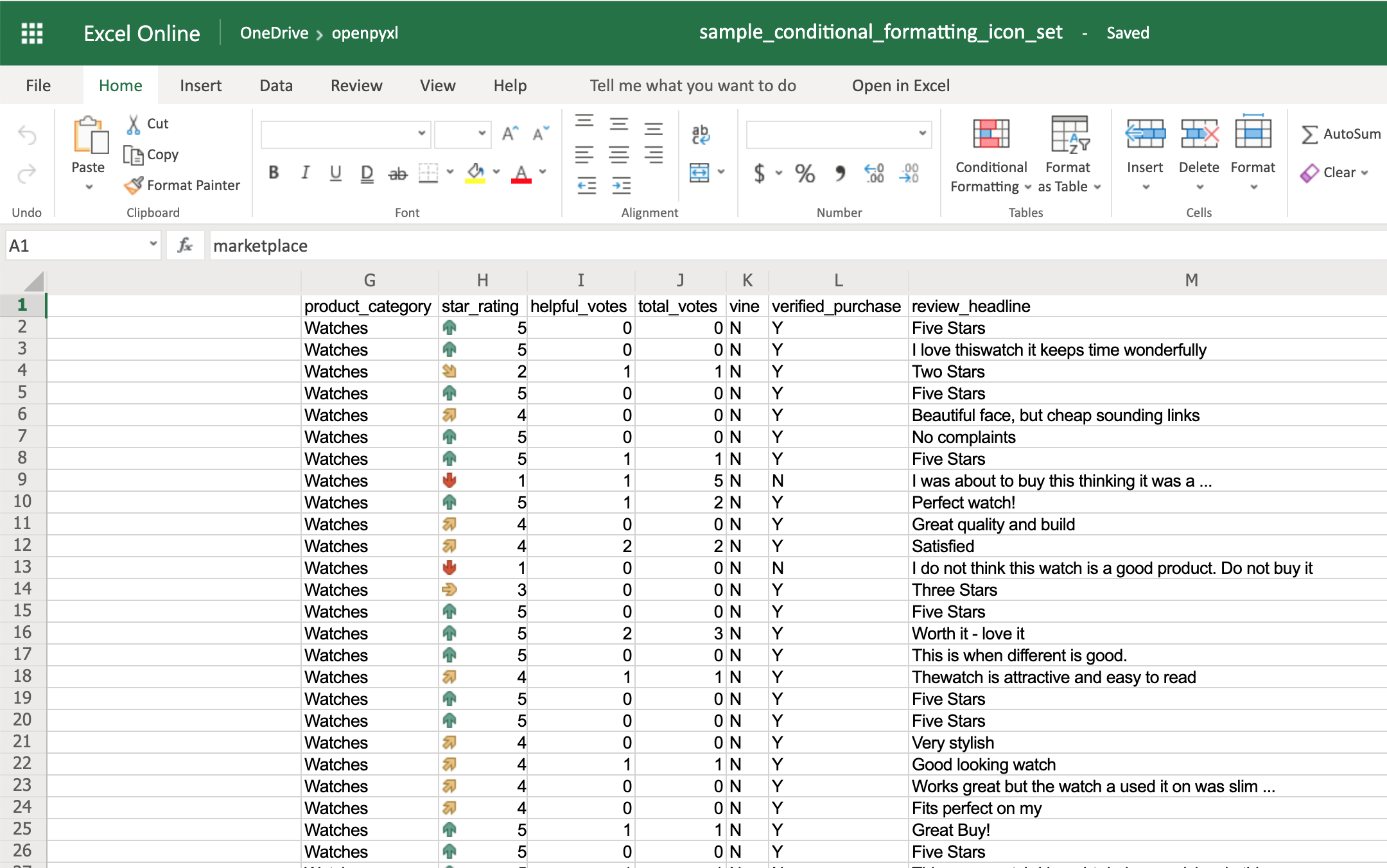
The openpyxl package has a full list of other icons you can use, besides the arrow.
Finally, the DataBar allows you to create progress bars:
>>> from openpyxl.formatting.rule import DataBarRule

>>> data_bar_rule = DataBarRule(start_type="num",
...                             start_value=1,
...                             end_type="num",
...                             end_value="5",
...                             color=colors.GREEN)
>>> sheet.conditional_formatting.add("H2:H100", data_bar_rule)
>>> workbook.save("sample_conditional_formatting_data_bar.xlsx")
You’ll now see a green progress bar that gets fuller the closer the star rating is to the number 5:
As you can see, there are a lot of cool things you can do with conditional formatting.
Here, you saw only a few examples of what you can achieve with it, but check the openpyxl documentation to see a bunch of other options.
Even though images are not something that you’ll often see in a spreadsheet, it’s quite cool to be able to add them. Maybe you can use it for branding purposes or to make spreadsheets more personal.
To be able to load images to a spreadsheet using openpyxl, you’ll have to install Pillow:
$ pip install Pillow
Apart from that, you’ll also need an image. For this example, you can grab the Real Python logo below and convert it from .webp to .png using an online converter such as cloudconvert.com, save the final file as logo.png, and copy it to the root folder where you’re running your examples:
![]()
Afterward, this is the code you need to import that image into the hello_word.xlsx spreadsheet:
from openpyxl import load_workbook
from openpyxl.drawing.image import Image

# Let's use the hello_world spreadsheet since it has less data
workbook = load_workbook(filename="hello_world.xlsx")
sheet = workbook.active

logo = Image("logo.png")

# A bit of resizing to not fill the whole spreadsheet with the logo
logo.height = 150
logo.width = 150

sheet.add_image(logo, "A3")
workbook.save(filename="hello_world_logo.xlsx")
You have an image on your spreadsheet! Here it is:
The image’s left top corner is on the cell you chose, in this case, A3.
Another powerful thing you can do with spreadsheets is create an incredible variety of charts.
Charts are a great way to visualize and understand loads of data quickly. There are a lot of different chart types: bar chart, pie chart, line chart, and so on. openpyxl has support for a lot of them.
Here, you’ll see only a couple of examples of charts because the theory behind it is the same for every single chart type:
Note: A few of the chart types that openpyxl currently doesn’t have support for are Funnel, Gantt, Pareto, Treemap, Waterfall, Map, and Sunburst.
For any chart you want to build, you’ll need to define the chart type: BarChart, LineChart, and so forth, plus the data to be used for the chart, which is called Reference.
Before you can build your chart, you need to define what data you want to see represented in it. Sometimes, you can use the dataset as is, but other times you need to massage the data a bit to get additional information.
Let’s start by building a new workbook with some sample data:
 1 from openpyxl import Workbook
 2 from openpyxl.chart import BarChart, Reference
 3
 4 workbook = Workbook()
 5 sheet = workbook.active
 6
 7 # Let's create some sample sales data
 8 rows = [
 9     ["Product", "Online", "Store"],
10     [1, 30, 45],
11     [2, 40, 30],
12     [3, 40, 25],
13     [4, 50, 30],
14     [5, 30, 25],
15     [6, 25, 35],
16     [7, 20, 40],
17 ]
18
19 for row in rows:
20     sheet.append(row)
Now you’re going to start by creating a bar chart that displays the total number of sales per product:
22 chart = BarChart()
23 data = Reference(worksheet=sheet,
24                  min_row=1,
25                  max_row=8,
26                  min_col=2,
27                  max_col=3)
28
29 chart.add_data(data, titles_from_data=True)
30 sheet.add_chart(chart, "E2")
31
32 workbook.save("chart.xlsx")
There you have it. Below, you can see a very straightforward bar chart showing the difference between online product sales online and in-store product sales:
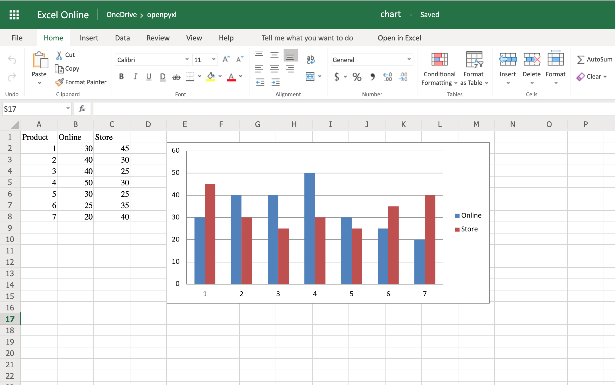
Like with images, the top left corner of the chart is on the cell you added the chart to. In your case, it was on cell E2.
Note: Depending on whether you’re using Microsoft Excel or an open-source alternative (LibreOffice or OpenOffice), the chart might look slightly different.
Try creating a line chart instead, changing the data a bit:
 1 import random
 2 from openpyxl import Workbook
 3 from openpyxl.chart import LineChart, Reference
 4
 5 workbook = Workbook()
 6 sheet = workbook.active
 7
 8 # Let's create some sample sales data
 9 rows = [
10     ["", "January", "February", "March", "April",
11     "May", "June", "July", "August", "September",
12      "October", "November", "December"],
13     [1, ],
14     [2, ],
15     [3, ],
16 ]
17
18 for row in rows:
19     sheet.append(row)
20
21 for row in sheet.iter_rows(min_row=2,
22                            max_row=4,
23                            min_col=2,
24                            max_col=13):
25     for cell in row:
26         cell.value = random.randrange(5, 100)
With the above code, you’ll be able to generate some random data regarding the sales of 3 different products across a whole year.
Once that’s done, you can very easily create a line chart with the following code:
28 chart = LineChart()
29 data = Reference(worksheet=sheet,
30                  min_row=2,
31                  max_row=4,
32                  min_col=1,
33                  max_col=13)
34
35 chart.add_data(data, from_rows=True, titles_from_data=True)
36 sheet.add_chart(chart, "C6")
37
38 workbook.save("line_chart.xlsx")
Here’s the outcome of the above piece of code:

One thing to keep in mind here is the fact that you’re using from_rows=True when adding the data. This argument makes the chart plot row by row instead of column by column.
In your sample data, you see that each product has a row with 12 values (1 column per month). That’s why you use from_rows. If you don’t pass that argument, by default, the chart tries to plot by column, and you’ll get a month-by-month comparison of sales.
Another difference that has to do with the above argument change is the fact that our Reference now starts from the first column, min_col=1, instead of the second one. This change is needed because the chart now expects the first column to have the titles.
There are a couple of other things you can also change regarding the style of the chart. For example, you can add specific categories to the chart:
cats = Reference(worksheet=sheet,
                 min_row=1,
                 max_row=1,
                 min_col=2,
                 max_col=13)
chart.set_categories(cats)
Add this piece of code before saving the workbook, and you should see the month names appearing instead of numbers:
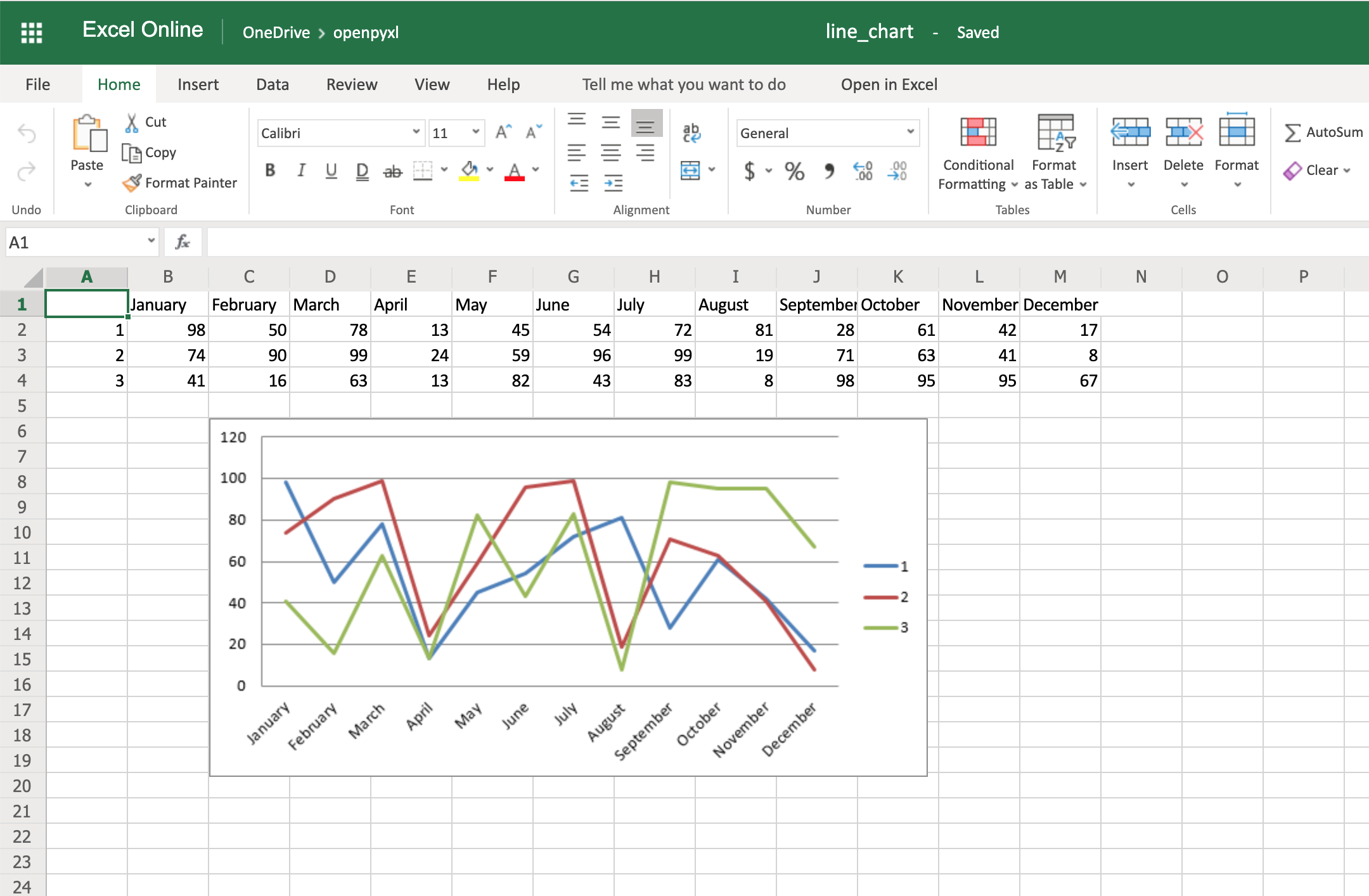
Code-wise, this is a minimal change. But in terms of the readability of the spreadsheet, this makes it much easier for someone to open the spreadsheet and understand the chart straight away.
Another thing you can do to improve the chart readability is to add an axis. You can do it using the attributes x_axis and y_axis:
chart.x_axis.title = "Months"
chart.y_axis.title = "Sales (per unit)"
This will generate a spreadsheet like the below one:
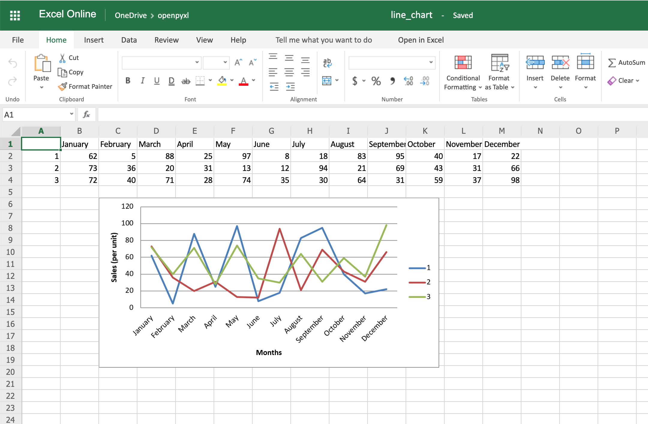
As you can see, small changes like the above make reading your chart a much easier and quicker task.
There is also a way to style your chart by using Excel’s default ChartStyle property. In this case, you have to choose a number between 1 and 48. Depending on your choice, the colors of your chart change as well:
# You can play with this by choosing any number between 1 and 48
chart.style = 24
With the style selected above, all lines have some shade of orange:

There is no clear documentation on what each style number looks like, but this spreadsheet has a few examples of the styles available.
Here’s the full code used to generate the line chart with categories, axis titles, and style:
import random
from openpyxl import Workbook
from openpyxl.chart import LineChart, Reference

workbook = Workbook()
sheet = workbook.active

# Let's create some sample sales data
rows = [
    ["", "January", "February", "March", "April",
    "May", "June", "July", "August", "September",
     "October", "November", "December"],
    [1, ],
    [2, ],
    [3, ],
]

for row in rows:
    sheet.append(row)

for row in sheet.iter_rows(min_row=2,
                           max_row=4,
                           min_col=2,
                           max_col=13):
    for cell in row:
        cell.value = random.randrange(5, 100)

# Create a LineChart and add the main data
chart = LineChart()
data = Reference(worksheet=sheet,
                           min_row=2,
                           max_row=4,
                           min_col=1,
                           max_col=13)
chart.add_data(data, titles_from_data=True, from_rows=True)

# Add categories to the chart
cats = Reference(worksheet=sheet,
                 min_row=1,
                 max_row=1,
                 min_col=2,
                 max_col=13)
chart.set_categories(cats)

# Rename the X and Y Axis
chart.x_axis.title = "Months"
chart.y_axis.title = "Sales (per unit)"

# Apply a specific Style
chart.style = 24

# Save!
sheet.add_chart(chart, "C6")
workbook.save("line_chart.xlsx")
There are a lot more chart types and customization you can apply, so be sure to check out the package documentation on this if you need some specific formatting.
You already saw how to convert an Excel spreadsheet’s data into Python classes, but now let’s do the opposite.
Let’s imagine you have a database and are using some Object-Relational Mapping (ORM) to map DB objects into Python classes. Now, you want to export those same objects into a spreadsheet.
Let’s assume the following data classes to represent the data coming from your database regarding product sales:
from dataclasses import dataclass
from typing import List

@dataclass
class Sale:
    id: str
    quantity: int

@dataclass
class Product:
    id: str
    name: str
    sales: List[Sale]
Now, let’s generate some random data, assuming the above classes are stored in a db_classes.py file:
 1 import random
 2
 3 # Ignore these for now. You'll use them in a sec ;)
 4 from openpyxl import Workbook
 5 from openpyxl.chart import LineChart, Reference
 6
 7 from db_classes import Product, Sale
 8
 9 products = []
10
11 # Let's create 5 products
12 for idx in range(1, 6):
13     sales = []
14
15     # Create 5 months of sales
16     for _ in range(5):
17         sale = Sale(quantity=random.randrange(5, 100))
18         sales.append(sale)
19
20     product = Product(id=str(idx),
21                       name="Product %s" % idx,
22                       sales=sales)
23     products.append(product)
By running this piece of code, you should get 5 products with 5 months of sales with a random quantity of sales for each month.
Now, to convert this into a spreadsheet, you need to iterate over the data and append it to the spreadsheet:
25 workbook = Workbook()
26 sheet = workbook.active
27
28 # Append column names first
29 sheet.append(["Product ID", "Product Name", "Month 1",
30               "Month 2", "Month 3", "Month 4", "Month 5"])
31
32 # Append the data
33 for product in products:
34     data = [product.id, product.name]
35     for sale in product.sales:
36         data.append(sale.quantity)
37     sheet.append(data)
That’s it. That should allow you to create a spreadsheet with some data coming from your database.
However, why not use some of that cool knowledge you gained recently to add a chart as well to display that data more visually?
All right, then you could probably do something like this:
38 chart = LineChart()
39 data = Reference(worksheet=sheet,
40                  min_row=2,
41                  max_row=6,
42                  min_col=2,
43                  max_col=7)
44
45 chart.add_data(data, titles_from_data=True, from_rows=True)
46 sheet.add_chart(chart, "B8")
47
48 cats = Reference(worksheet=sheet,
49                  min_row=1,
50                  max_row=1,
51                  min_col=3,
52                  max_col=7)
53 chart.set_categories(cats)
54
55 chart.x_axis.title = "Months"
56 chart.y_axis.title = "Sales (per unit)"
57
58 workbook.save(filename="oop_sample.xlsx")
Now we’re talking! Here’s a spreadsheet generated from database objects and with a chart and everything:
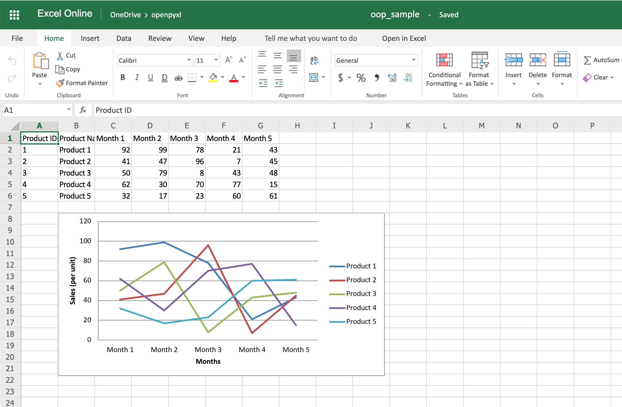
That’s a great way for you to wrap up your new knowledge of charts!
Even though you can use Pandas to handle Excel files, there are few things that you either can’t accomplish with Pandas or that you’d be better off just using openpyxl directly.
For example, some of the advantages of using openpyxl are the ability to easily customize your spreadsheet with styles, conditional formatting, and such.
But guess what, you don’t have to worry about picking. In fact, openpyxl has support for both converting data from a Pandas DataFrame into a workbook or the opposite, converting an openpyxl workbook into a Pandas DataFrame.
Note: If you’re new to Pandas, check our course on Pandas DataFrames beforehand.
First things first, remember to install the pandas package:
$ pip install pandas
Then, let’s create a sample DataFrame:
 1 import pandas as pd
 2
 3 data = {
 4     "Product Name": ["Product 1", "Product 2"],
 5     "Sales Month 1": [10, 20],
 6     "Sales Month 2": [5, 35],
 7 }
 8 df = pd.DataFrame(data)
Now that you have some data, you can use .dataframe_to_rows() to convert it from a DataFrame into a worksheet:
10 from openpyxl import Workbook
11 from openpyxl.utils.dataframe import dataframe_to_rows
12
13 workbook = Workbook()
14 sheet = workbook.active
15
16 for row in dataframe_to_rows(df, index=False, header=True):
17     sheet.append(row)
18
19 workbook.save("pandas.xlsx")
You should see a spreadsheet that looks like this:
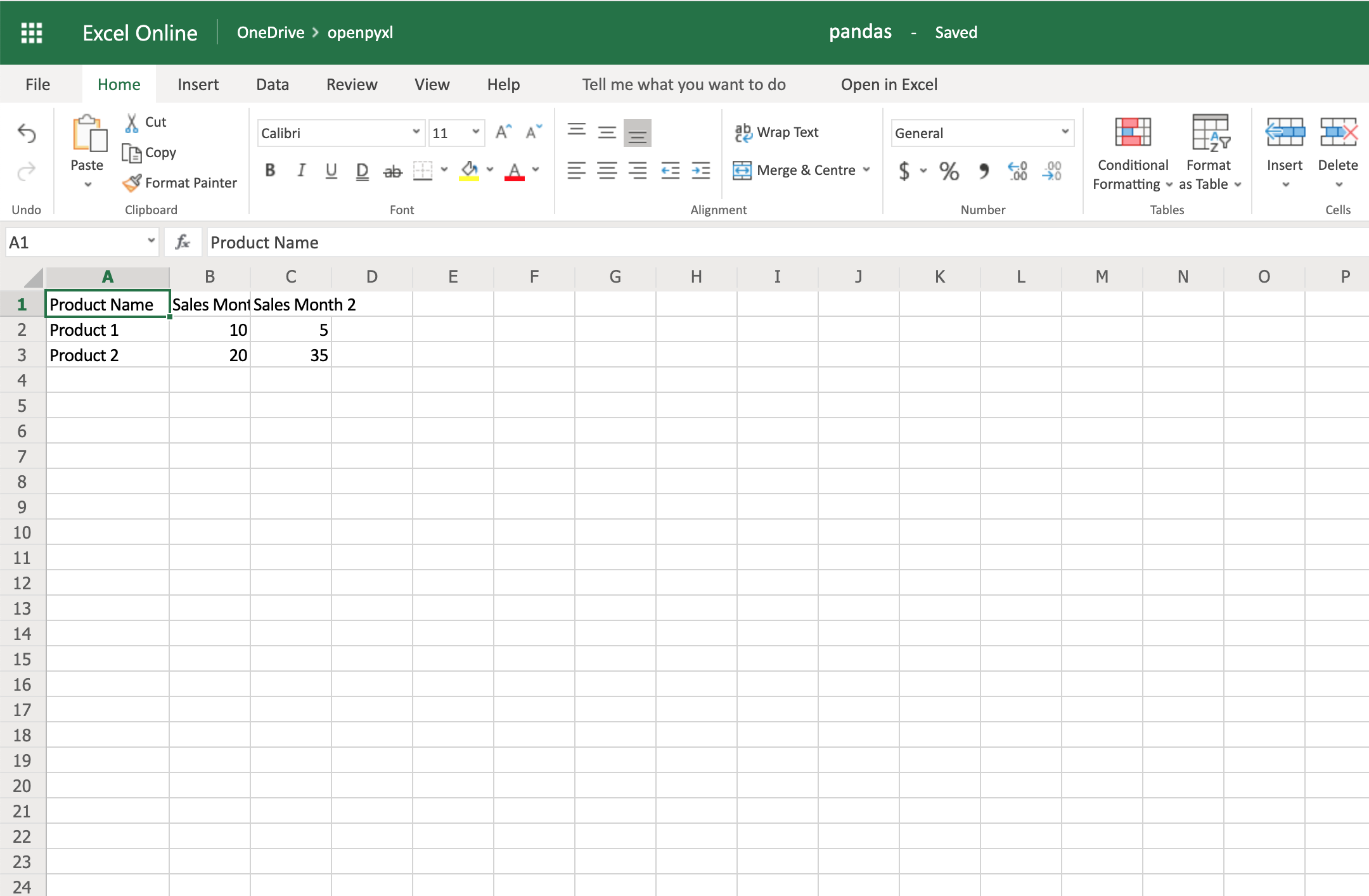
If you want to add the DataFrame’s index, you can change index=True, and it adds each row’s index into your spreadsheet.
On the other hand, if you want to convert a spreadsheet into a DataFrame, you can also do it in a very straightforward way like so:
import pandas as pd
from openpyxl import load_workbook

workbook = load_workbook(filename="sample.xlsx")
sheet = workbook.active

values = sheet.values
df = pd.DataFrame(values)
Alternatively, if you want to add the correct headers and use the review ID as the index, for example, then you can also do it like this instead:
import pandas as pd
from openpyxl import load_workbook
from mapping import REVIEW_ID

workbook = load_workbook(filename="sample.xlsx")
sheet = workbook.active

data = sheet.values

# Set the first row as the columns for the DataFrame
cols = next(data)
data = list(data)

# Set the field "review_id" as the indexes for each row
idx = [row[REVIEW_ID] for row in data]

df = pd.DataFrame(data, index=idx, columns=cols)
Using indexes and columns allows you to access data from your DataFrame easily:
>>> df.columns
Index(['marketplace', 'customer_id', 'review_id', 'product_id',
       'product_parent', 'product_title', 'product_category', 'star_rating',
       'helpful_votes', 'total_votes', 'vine', 'verified_purchase',
       'review_headline', 'review_body', 'review_date'],
      dtype='object')

>>> # Get first 10 reviews' star rating
>>> df["star_rating"][:10]
R3O9SGZBVQBV76    5
RKH8BNC3L5DLF     5
R2HLE8WKZSU3NL    2
R31U3UH5AZ42LL    5
R2SV659OUJ945Y    4
RA51CP8TR5A2L     5
RB2Q7DLDN6TH6     5
R2RHFJV0UYBK3Y    1
R2Z6JOQ94LFHEP    5
RX27XIIWY5JPB     4
Name: star_rating, dtype: int64

>>> # Grab review with id "R2EQL1V1L6E0C9", using the index
>>> df.loc["R2EQL1V1L6E0C9"]
marketplace               US
customer_id         15305006
review_id     R2EQL1V1L6E0C9
product_id        B004LURNO6
product_parent     892860326
review_headline   Five Stars
review_body          Love it
review_date       2015-08-31
Name: R2EQL1V1L6E0C9, dtype: object
There you go, whether you want to use openpyxl to prettify your Pandas dataset or use Pandas to do some hardcore algebra, you now know how to switch between both packages.
Phew, after that long read, you now know how to work with spreadsheets in Python! You can rely on openpyxl, your trustworthy companion, to:
There are a few other things you can do with openpyxl that might not have been covered in this tutorial, but you can always check the package’s official documentation website to learn more about it. You can even venture into checking its source code and improving the package further.
Feel free to leave any comments below if you have any questions, or if there’s any section you’d love to hear more about.
Download Dataset: Click here to download the dataset for the openpyxl exercise you'll be following in this tutorial.
[ Improve Your Python With 🐍 Python Tricks 💌 – Get a short & sweet Python Trick delivered to your inbox every couple of days. >> Click here to learn more and see examples ]
# datePublished: #Mon Aug 26 14:00:00 2019# dateUpdated: #Mon Aug 26 14:00:00 2019# # Person begin #################### name: #Real Python# # Person end ###################### # Item end ######################## # Item begin ###################### id: #https://realpython.com/cpython-source-code-guide/# title: #Your Guide to the CPython Source Code# link: #https://realpython.com/cpython-source-code-guide/# description: #In this detailed Python tutorial, you'll explore the CPython source code. By following this step-by-step walkthrough, you'll take a deep dive into how the CPython compiler works and how your Python code gets executed.# content: #Are there certain parts of Python that just seem magic? Like how are dictionaries so much faster than looping over a list to find an item. How does a generator remember the state of the variables each time it yields a value and why do you never have to allocate memory like other languages? It turns out, CPython, the most popular Python runtime is written in human-readable C and Python code. This tutorial will walk you through the CPython source code.
You’ll cover all the concepts behind the internals of CPython, how they work and visual explanations as you go.
You’ll learn how to:
Yes, this is a very long article. If you just made yourself a fresh cup of tea, coffee or your favorite beverage, it’s going to be cold by the end of Part 1.
This tutorial is split into five parts. Take your time for each part and make sure you try out the demos and the interactive components. You can feel a sense of achievement that you grasp the core concepts of Python that can make you a better Python programmer.
Free Bonus: 5 Thoughts On Python Mastery, a free course for Python developers that shows you the roadmap and the mindset you'll need to take your Python skills to the next level.
When you type python at the console or install a Python distribution from python.org, you are running CPython. CPython is one of the many Python runtimes, maintained and written by different teams of developers. Some other runtimes you may have heard are PyPy, Cython, and Jython.
The unique thing about CPython is that it contains both a runtime and the shared language specification that all Python runtimes use. CPython is the “official,” or reference implementation of Python.
The Python language specification is the document that the description of the Python language. For example, it says that assert is a reserved keyword, and that [] is used for indexing, slicing, and creating empty lists.
Think about what you expect to be inside the Python distribution on your computer:
python without a file or module, it gives an interactive prompt.json.pip.unittest library.These are all part of the CPython distribution. There’s a lot more than just a compiler.
Note: This article is written against version 3.8.0b4 of the CPython source code.
The CPython source distribution comes with a whole range of tools, libraries, and components. We’ll explore those in this article. First we are going to focus on the compiler.
To download a copy of the CPython source code, you can use git to pull the latest version to a working copy locally:
git clone https://github.com/python/cpython
cd cpython
git checkout v3.8.0b4
Note: If you don’t have Git available, you can download the source in a ZIP file directly from the GitHub website.
Inside of the newly downloaded cpython directory, you will find the following subdirectories:
cpython/
│
├── Doc      ← Source for the documentation
├── Grammar  ← The computer-readable language definition
├── Include  ← The C header files
├── Lib      ← Standard library modules written in Python
├── Mac      ← macOS support files
├── Misc     ← Miscellaneous files
├── Modules  ← Standard Library Modules written in C
├── Objects  ← Core types and the object model
├── Parser   ← The Python parser source code
├── PC       ← Windows build support files
├── PCbuild  ← Windows build support files for older Windows versions
├── Programs ← Source code for the python executable and other binaries
├── Python   ← The CPython interpreter source code
└── Tools    ← Standalone tools useful for building or extending Python
Next, we’ll compile CPython from the source code. This step requires a C compiler, and some build tools, which depend on the operating system you’re using.
Compiling CPython on macOS is straightforward. You will first need the essential C compiler toolkit. The Command Line Development Tools is an app that you can update in macOS through the App Store. You need to perform the initial installation on the terminal.
To open up a terminal in macOS, go to the Launchpad, then Other then choose the Terminal app. You will want to save this app to your Dock, so right-click the Icon and select Keep in Dock.
Now, within the terminal, install the C compiler and toolkit by running the following:
$ xcode-select --install
This command will pop up with a prompt to download and install a set of tools, including Git, Make, and the GNU C compiler.
You will also need a working copy of OpenSSL to use for fetching packages from the PyPi.org website. If you later plan on using this build to install additional packages, SSL validation is required.
The simplest way to install OpenSSL on macOS is by using HomeBrew. If you already have HomeBrew installed, you can install the dependencies for CPython with the brew install command:
$ brew install openssl xz zlib
Now that you have the dependencies, you can run the configure script, enabling SSL support by discovering the location that HomeBrew installed to and enabling the debug hooks --with-pydebug:
$ CPPFLAGS="-I$(brew --prefix zlib)/include" \
 LDFLAGS="-L$(brew --prefix zlib)/lib" \
 ./configure --with-openssl=$(brew --prefix openssl) --with-pydebug
This will generate a Makefile in the root of the repository that you can use to automate the build process. The ./configure step only needs to be run once. You can build the CPython binary by running:
$ make -j2 -s
The -j2 flag allows make to run 2 jobs simultaneously. If you have 4 cores, you can change this to 4. The -s flag stops the Makefile from printing every command it runs to the console. You can remove this, but the output is very verbose.
During the build, you may receive some errors, and in the summary, it will notify you that not all packages could be built. For example, _dbm, _sqlite3, _uuid, nis, ossaudiodev, spwd, and _tkinter would fail to build with this set of instructions. That’s okay if you aren’t planning on developing against those packages. If you are, then check out the dev guide website for more information.
The build will take a few minutes and generate a binary called python.exe. Every time you make changes to the source code, you will need to re-run make with the same flags.
The python.exe binary is the debug binary of CPython. Execute python.exe to see a working REPL:
$ ./python.exe
Python 3.8.0b4 (tags/v3.8.0b4:d93605de72, Aug 30 2019, 10:00:03)
[Clang 10.0.1 (clang-1001.0.46.4)] on darwin
Type "help", "copyright", "credits" or "license" for more information.
>>>
Note:
Yes, that’s right, the macOS build has a file extension for .exe. This is not because it’s a Windows binary. Because macOS has a case-insensitive filesystem and when working with the binary, the developers didn’t want people to accidentally refer to the directory Python/ so .exe was appended to avoid ambiguity.
If you later run make install or make altinstall, it will rename the file back to python.
For Linux, the first step is to download and install make, gcc, configure, and pkgconfig.
For Fedora Core, RHEL, CentOS, or other yum-based systems:
$ sudo yum install yum-utils
For Debian, Ubuntu, or other apt-based systems:
$ sudo apt install build-essential
Then install the required packages, for Fedora Core, RHEL, CentOS or other yum-based systems:
$ sudo yum-builddep python3
For Debian, Ubuntu, or other apt-based systems:
$ sudo apt install libssl-dev zlib1g-dev libncurses5-dev \
  libncursesw5-dev libreadline-dev libsqlite3-dev libgdbm-dev \
  libdb5.3-dev libbz2-dev libexpat1-dev liblzma-dev libffi-dev
Now that you have the dependencies, you can run the configure script, enabling the debug hooks --with-pydebug:
$ ./configure --with-pydebug
Review the output to ensure that OpenSSL support was marked as YES. Otherwise, check with your distribution for instructions on installing the headers for OpenSSL.
Next, you can build the CPython binary by running the generated Makefile:
$ make -j2 -s
During the build, you may receive some errors, and in the summary, it will notify you that not all packages could be built. That’s okay if you aren’t planning on developing against those packages. If you are, then check out the dev guide website for more information.
The build will take a few minutes and generate a binary called python. This is the debug binary of CPython. Execute ./python to see a working REPL:
$ ./python
Python 3.8.0b4 (tags/v3.8.0b4:d93605de72, Aug 30 2019, 10:00:03)
[Clang 10.0.1 (clang-1001.0.46.4)] on darwin
Type "help", "copyright", "credits" or "license" for more information.
>>>
Inside the PC folder is a Visual Studio project file for building and exploring CPython. To use this, you need to have Visual Studio installed on your PC.
The newest version of Visual Studio, Visual Studio 2019, makes it easier to work with Python and the CPython source code, so it is recommended for use in this tutorial. If you already have Visual Studio 2017 installed, that would also work fine.
None of the paid features are required for compiling CPython or this tutorial. You can use the Community edition of Visual Studio, which is available for free from Microsoft’s Visual Studio website.
Once you’ve downloaded the installer, you’ll be asked to select which components you want to install. The bare minimum for this tutorial is:
Any other optional features can be deselected if you want to be more conscientious with disk space:

The installer will then download and install all of the required components. The installation could take an hour, so you may want to read on and come back to this section.
Once the installer has completed, click the Launch button to start Visual Studio. You will be prompted to sign in. If you have a Microsoft account you can log in, or skip that step.
Once Visual Studio starts, you will be prompted to Open a Project. A shortcut to getting started with the Git configuration and cloning CPython is to choose the Clone or check out code option:

For the project URL, type https://github.com/python/cpython to clone:
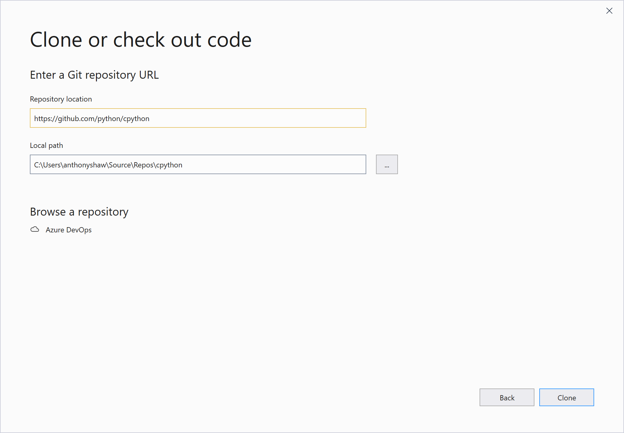
Visual Studio will then download a copy of CPython from GitHub using the version of Git bundled with Visual Studio. This step also saves you the hassle of having to install Git on Windows. The download may take 10 minutes.
Once the project has downloaded, you need to point it to the pcbuild Solution file, by clicking on Solutions and Projects and selecting pcbuild.sln:
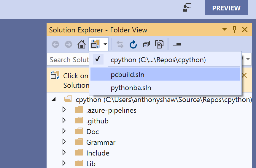
When the solution is loaded, it will prompt you to retarget the project’s inside the solution to the version of the C/C++ compiler you have installed. Visual Studio will also target the version of the Windows SDK you have installed.
Ensure that you change the Windows SDK version to the newest installed version and the platform toolset to the latest version. If you missed this window, you can right-click on the Solution in the Solutions and Projects window and click Retarget Solution.
Once this is complete, you need to download some source files to be able to build the whole CPython package. Inside the PCBuild folder there is a .bat file that automates this for you. Open up a command-line prompt inside the downloaded PCBuild and run get_externals.bat:
 > get_externals.bat
Using py -3.7 (found 3.7 with py.exe)
Fetching external libraries...
Fetching bzip2-1.0.6...
Fetching sqlite-3.21.0.0...
Fetching xz-5.2.2...
Fetching zlib-1.2.11...
Fetching external binaries...
Fetching openssl-bin-1.1.0j...
Fetching tcltk-8.6.9.0...
Finished.
Next, back within Visual Studio, build CPython by pressing Ctrl+Shift+B, or choosing Build Solution from the top menu. If you receive any errors about the Windows SDK being missing, make sure you set the right targeting settings in the Retarget Solution window. You should also see Windows Kits inside your Start Menu, and Windows Software Development Kit inside of that menu.
The build stage could take 10 minutes or more for the first time. Once the build is completed, you may see a few warnings that you can ignore and eventual completion.
To start the debug version of CPython, press F5 and CPython will start in Debug mode straight into the REPL:

Once this is completed, you can run the Release build by changing the build configuration from Debug to Release on the top menu bar and rerunning Build Solution again.
You now have both Debug and Release versions of the CPython binary within PCBuild\win32\.
You can set up Visual Studio to be able to open a REPL with either the Release or Debug build by choosing Tools->Python->Python Environments from the top menu:

Then click Add Environment and then target the Debug or Release binary. The Debug binary will end in _d.exe, for example, python_d.exe and pythonw_d.exe. You will most likely want to use the debug binary as it comes with Debugging support in Visual Studio and will be useful for this tutorial.
In the Add Environment window, target the python_d.exe file as the interpreter inside the PCBuild/win32 and the pythonw_d.exe as the windowed interpreter:

Now, you can start a REPL session by clicking Open Interactive Window in the Python Environments window and you will see the REPL for the compiled version of Python:

During this tutorial there will be REPL sessions with example commands. I encourage you to use the Debug binary to run these REPL sessions in case you want to put in any breakpoints within the code.
Lastly, to make it easier to navigate the code, in the Solution View, click on the toggle button next to the Home icon to switch to Folder view:

Now you have a version of CPython compiled and ready to go, let’s find out how the CPython compiler works.
The purpose of a compiler is to convert one language into another. Think of a compiler like a translator. You would hire a translator to listen to you speaking in English and then speak in Japanese:

Some compilers will compile into a low-level machine code which can be executed directly on a system. Other compilers will compile into an intermediary language, to be executed by a virtual machine.
One important decision to make when choosing a compiler is the system portability requirements. Java and .NET CLR will compile into an Intermediary Language so that the compiled code is portable across multiple systems architectures. C, Go, C++, and Pascal will compile into a low-level executable that will only work on systems similar to the one it was compiled.
Because Python applications are typically distributed as source code, the role of the Python runtime is to convert the Python source code and execute it in one step. Internally, the CPython runtime does compile your code. A popular misconception is that Python is an interpreted language. It is actually compiled.
Python code is not compiled into machine-code. It is compiled into a special low-level intermediary language called bytecode that only CPython understands. This code is stored in .pyc files in a hidden directory and cached for execution. If you run the same Python application twice without changing the source code, it’ll always be much faster the second time. This is because it loads the compiled bytecode and executes it directly.
The C in CPython is a reference to the C programming language, implying that this Python distribution is written in the C language.
This statement is largely true: the compiler in CPython is written in pure C. However, many of the standard library modules are written in pure Python or a combination of C and Python.
So why is CPython written in C and not Python?
The answer is located in how compilers work. There are two types of compiler:
If you’re writing a new programming language from scratch, you need an executable application to compile your compiler! You need a compiler to execute anything, so when new languages are developed, they’re often written first in an older, more established language.
A good example would be the Go programming language. The first Go compiler was written in C, then once Go could be compiled, the compiler was rewritten in Go.
CPython kept its C heritage: many of the standard library modules, like the ssl module or the sockets module, are written in C to access low-level operating system APIs.
The APIs in the Windows and Linux kernels for creating network sockets, working with the filesystem or interacting with the display are all written in C. It made sense for Python’s extensibility layer to be focused on the C language. Later in this article, we will cover the Python Standard Library and the C modules.
There is a Python compiler written in Python called PyPy. PyPy’s logo is an Ouroboros to represent the self-hosting nature of the compiler.
Another example of a cross-compiler for Python is Jython. Jython is written in Java and compiles from Python source code into Java bytecode. In the same way that CPython makes it easy to import C libraries and use them from Python, Jython makes it easy to import and reference Java modules and classes.
Contained within the CPython source code is the definition of the Python language. This is the reference specification used by all the Python interpreters.
The specification is in both human-readable and machine-readable format. Inside the documentation is a detailed explanation of the Python language, what is allowed, and how each statement should behave.
Located inside the Doc/reference directory are reStructuredText explanations of each of the features in the Python language. This forms the official Python reference guide on docs.python.org.
Inside the directory are the files you need to understand the whole language, structure, and keywords:
cpython/Doc/reference
|
├── compound_stmts.rst
├── datamodel.rst
├── executionmodel.rst
├── expressions.rst
├── grammar.rst
├── import.rst
├── index.rst
├── introduction.rst
├── lexical_analysis.rst
├── simple_stmts.rst
└── toplevel_components.rst
Inside compound_stmts.rst, the documentation for compound statements, you can see a simple example defining the with statement.
The with statement can be used in multiple ways in Python, the simplest being the instantiation of a context-manager and a nested block of code:
with x():
   ...
You can assign the result to a variable using the as keyword:
with x() as y:
   ...
You can also chain context managers together with a comma:
with x() as y, z() as jk:
   ...
Next, we’ll explore the computer-readable documentation of the Python language.
The documentation contains the human-readable specification of the language, and the machine-readable specification is housed in a single file, Grammar/Grammar.
The Grammar file is written in a context-notation called Backus-Naur Form (BNF). BNF is not specific to Python and is often used as the notation for grammars in many other languages.
The concept of grammatical structure in a programming language is inspired by Noam Chomsky’s work on Syntactic Structures in the 1950s!
Python’s grammar file uses the Extended-BNF (EBNF) specification with regular-expression syntax. So, in the grammar file you can use:
* for repetition+ for at-least-once repetition[] for optional parts| for alternatives() for groupingIf you search for the with statement in the grammar file, at around line 80 you’ll see the definitions for the with statement:
with_stmt: 'with' with_item (',' with_item)*  ':' suite
with_item: test ['as' expr]
Anything in quotes is a string literal, which is how keywords are defined. So the with_stmt is specified as:
withwith_item, which is a test and (optionally), the word as, and an expression:suiteThere are references to some other definitions in these two lines:
suite refers to a block of code with one or multiple statementstest refers to a simple statement that is evaluatedexpr refers to a simple expressionIf you want to explore those in detail, the whole of the Python grammar is defined in this single file.
If you want to see a recent example of how grammar is used, in PEP 572 the colon equals operator was added to the grammar file in this Git commit.
pgenThe grammar file itself is never used by the Python compiler. Instead, a parser table created by a tool called pgen is used. pgen reads the grammar file and converts it into a parser table. If you make changes to the grammar file, you must regenerate the parser table and recompile Python.
Note: The pgen application was rewritten in Python 3.8 from C to pure Python.
To see pgen in action, let’s change part of the Python grammar. Around line 51 you will see the definition of a pass statement:
pass_stmt: 'pass'
Change that line to accept the keyword 'pass' or 'proceed' as keywords:
pass_stmt: 'pass' | 'proceed'
Now you need to rebuild the grammar files.
On macOS and Linux, run make regen-grammar to run pgen over the altered grammar file. For Windows, there is no officially supported way of running pgen. However, you can clone my fork and run build.bat --regen from within the PCBuild directory.
You should see an output similar to this, showing that the new Include/graminit.h and Python/graminit.c files have been generated:
# Regenerate Doc/library/token-list.inc from Grammar/Tokens
# using Tools/scripts/generate_token.py
...
python3 ./Tools/scripts/update_file.py ./Include/graminit.h ./Include/graminit.h.new
python3 ./Tools/scripts/update_file.py ./Python/graminit.c ./Python/graminit.c.new
Note: pgen works by converting the EBNF statements into a Non-deterministic Finite Automaton (NFA), which is then turned into a Deterministic Finite Automaton (DFA).
The DFAs are used by the parser as parsing tables in a special way that’s unique to CPython. This technique was formed at Stanford University and developed in the 1980s, just before the advent of Python.
With the regenerated parser tables, you need to recompile CPython to see the new syntax. Use the same compilation steps you used earlier for your operating system.
If the code compiled successfully, you can execute your new CPython binary and start a REPL.
In the REPL, you can now try defining a function and instead of using the pass statement, use the proceed keyword alternative that you compiled into the Python grammar:
Python 3.8.0b4 (tags/v3.8.0b4:d93605de72, Aug 30 2019, 10:00:03)
[Clang 10.0.1 (clang-1001.0.46.4)] on darwin
Type "help", "copyright", "credits" or "license" for more information.
>>> def example():
...    proceed
...
>>> example()
Well done! You’ve changed the CPython syntax and compiled your own version of CPython. Ship it!
Next, we’ll explore tokens and their relationship to grammar.
Alongside the grammar file in the Grammar folder is a Tokens file, which contains each of the unique types found as a leaf node in a parse tree. We will cover parser trees in depth later.
Each token also has a name and a generated unique ID. The names are used to make it simpler to refer to in the tokenizer.
Note: The Tokens file is a new feature in Python 3.8.
For example, the left parenthesis is called LPAR, and semicolons are called SEMI. You’ll see these tokens later in the article:
LPAR                    '('
RPAR                    ')'
LSQB                    '['
RSQB                    ']'
COLON                   ':'
COMMA                   ','
SEMI                    ';'
As with the Grammar file, if you change the Tokens file, you need to run pgen again.
To see tokens in action, you can use the tokenize module in CPython. Create a simple Python script called test_tokens.py:
# Hello world!
def my_function():
   proceed
For the rest of this tutorial, ./python.exe will refer to the compiled version of CPython. However, the actual command will depend on your system.
For Windows:
> python.exe
For Linux:
> ./python
For macOS:
> ./python.exe
Then pass this file through a module built into the standard library called tokenize. You will see the list of tokens, by line and character. Use the -e flag to output the exact token name:
$ ./python.exe -m tokenize -e test_tokens.py

0,0-0,0:            ENCODING       'utf-8'
1,0-1,14:           COMMENT        '# Hello world!'
1,14-1,15:          NL             '\n'
2,0-2,3:            NAME           'def'
2,4-2,15:           NAME           'my_function'
2,15-2,16:          LPAR           '('
2,16-2,17:          RPAR           ')'
2,17-2,18:          COLON          ':'
2,18-2,19:          NEWLINE        '\n'
3,0-3,3:            INDENT         '   '
3,3-3,7:            NAME           'proceed'
3,7-3,8:            NEWLINE        '\n'
4,0-4,0:            DEDENT         ''
4,0-4,0:            ENDMARKER      ''
In the output, the first column is the range of the line/column coordinates, the second column is the name of the token, and the final column is the value of the token.
In the output, the tokenize module has implied some tokens that were not in the file. The ENCODING token for utf-8, and a blank line at the end, giving DEDENT to close the function declaration and an ENDMARKER to end the file.
It is best practice to have a blank line at the end of your Python source files. If you omit it, CPython adds it for you, with a tiny performance penalty.
The tokenize module is written in pure Python and is located in Lib/tokenize.py within the CPython source code.
Important: There are two tokenizers in the CPython source code: one written in Python, demonstrated here, and another written in C. The tokenizer written in Python is meant as a utility, and the one written in C is used by the Python compiler. They have identical output and behavior. The version written in C is designed for performance and the module in Python is designed for debugging.
To see a verbose readout of the C tokenizer, you can run Python with the -d flag. Using the test_tokens.py script you created earlier, run it with the following:
$ ./python.exe -d test_tokens.py

Token NAME/'def' ... It's a keyword
 DFA 'file_input', state 0: Push 'stmt'
 DFA 'stmt', state 0: Push 'compound_stmt'
 DFA 'compound_stmt', state 0: Push 'funcdef'
 DFA 'funcdef', state 0: Shift.
Token NAME/'my_function' ... It's a token we know
 DFA 'funcdef', state 1: Shift.
Token LPAR/'(' ... It's a token we know
 DFA 'funcdef', state 2: Push 'parameters'
 DFA 'parameters', state 0: Shift.
Token RPAR/')' ... It's a token we know
 DFA 'parameters', state 1: Shift.
  DFA 'parameters', state 2: Direct pop.
Token COLON/':' ... It's a token we know
 DFA 'funcdef', state 3: Shift.
Token NEWLINE/'' ... It's a token we know
 DFA 'funcdef', state 5: [switch func_body_suite to suite] Push 'suite'
 DFA 'suite', state 0: Shift.
Token INDENT/'' ... It's a token we know
 DFA 'suite', state 1: Shift.
Token NAME/'proceed' ... It's a keyword
 DFA 'suite', state 3: Push 'stmt'
...
  ACCEPT.
In the output, you can see that it highlighted proceed as a keyword. In the next chapter, we’ll see how executing the Python binary gets to the tokenizer and what happens from there to execute your code.
Now that you have an overview of the Python grammar and the relationship between tokens and statements, there is a way to convert the pgen output into an interactive graph.
Here is a screenshot of the Python 3.8a2 grammar:

The Python package used to generate this graph, instaviz, will be covered in a later chapter.
Throughout this article, you will see references to a PyArena object. The arena is one of CPython’s memory management structures. The code is within Python/pyarena.c and contains a wrapper around C’s memory allocation and deallocation functions.
In a traditionally written C program, the developer should allocate memory for data structures before writing into that data. This allocation marks the memory as belonging to the process with the operating system.
It is also up to the developer to deallocate, or “free,” the allocated memory when its no longer being used and return it to the operating system’s block table of free memory. If a process allocates memory for a variable, say within a function or loop, when that function has completed, the memory is not automatically given back to the operating system in C. So if it hasn’t been explicitly deallocated in the C code, it causes a memory leak. The process will continue to take more memory each time that function runs until eventually, the system runs out of memory, and crashes!
Python takes that responsibility away from the programmer and uses two algorithms: a reference counter and a garbage collector.
Whenever an interpreter is instantiated, a PyArena is created and attached one of the fields in the interpreter. During the lifecycle of a CPython interpreter, many arenas could be allocated. They are connected with a linked list. The arena stores a list of pointers to Python Objects as a PyListObject. Whenever a new Python object is created, a pointer to it is added using PyArena_AddPyObject(). This function call stores a pointer in the arena’s list, a_objects.
Even though Python doesn’t have pointers, there are some interesting techniques to simulate the behavior of pointers.
The PyArena serves a second function, which is to allocate and reference a list of raw memory blocks. For example, a PyList would need extra memory if you added thousands of additional values. The PyList object’s C code does not allocate memory directly. The object gets raw blocks of memory from the PyArena by calling PyArena_Malloc() from the PyObject with the required memory size. This task is completed by another abstraction in Objects/obmalloc.c. In the object allocation module, memory can be allocated, freed, and reallocated for a Python Object.
A linked list of allocated blocks is stored inside the arena, so that when an interpreter is stopped, all managed memory blocks can be deallocated in one go using PyArena_Free().
Take the PyListObject example. If you were to .append() an object to the end of a Python list, you don’t need to reallocate the memory used in the existing list beforehand. The .append() method calls list_resize() which handles memory allocation for lists. Each list object keeps a list of the amount of memory allocated. If the item you’re appending will fit inside the existing free memory, it is simply added. If the list needs more memory space, it is expanded. Lists are expanded in length as 0, 4, 8, 16, 25, 35, 46, 58, 72, 88.
PyMem_Realloc() is called to expand the memory allocated in a list. PyMem_Realloc() is an API wrapper for pymalloc_realloc().
Python also has a special wrapper for the C call malloc(), which sets the max size of the memory allocation to help prevent buffer overflow errors (See PyMem_RawMalloc()).
In summary:
PyMem_RawAlloc().PyArena.PyArena also stores a linked-list of allocated memory blocks.More information on the API is detailed on the CPython documentation.
To create a variable in Python, you have to assign a value to a uniquely named variable:
my_variable = 180392
Whenever a value is assigned to a variable in Python, the name of the variable is checked within the locals and globals scope to see if it already exists.
Because my_variable is not already within the locals() or globals() dictionary, this new object is created, and the value is assigned as being the numeric constant 180392.
There is now one reference to my_variable, so the reference counter for my_variable is incremented by 1.
You will see function calls Py_INCREF() and Py_DECREF() throughout the C source code for CPython. These functions increment and decrement the count of references to that object.
References to an object are decremented when a variable falls outside of the scope in which it was declared. Scope in Python can refer to a function or method, a comprehension, or a lambda function. These are some of the more literal scopes, but there are many other implicit scopes, like passing variables to a function call.
The handling of incrementing and decrementing references based on the language is built into the CPython compiler and the core execution loop, ceval.c, which we will cover in detail later in this article.
Whenever Py_DECREF() is called, and the counter becomes 0, the PyObject_Free() function is called. For that object PyArena_Free() is called for all of the memory that was allocated.
How often does your garbage get collected? Weekly, or fortnightly?
When you’re finished with something, you discard it and throw it in the trash. But that trash won’t get collected straight away. You need to wait for the garbage trucks to come and pick it up.
CPython has the same principle, using a garbage collection algorithm. CPython’s garbage collector is enabled by default, happens in the background and works to deallocate memory that’s been used for objects which are no longer in use.
Because the garbage collection algorithm is a lot more complex than the reference counter, it doesn’t happen all the time, otherwise, it would consume a huge amount of CPU resources. It happens periodically, after a set number of operations.
CPython’s standard library comes with a Python module to interface with the arena and the garbage collector, the gc module. Here’s how to use the gc module in debug mode:
>>> import gc
>>> gc.set_debug(gc.DEBUG_STATS)
This will print the statistics whenever the garbage collector is run.
You can get the threshold after which the garbage collector is run by calling get_threshold():
>>> gc.get_threshold()
(700, 10, 10)
You can also get the current threshold counts:
>>> gc.get_count()
(688, 1, 1)
Lastly, you can run the collection algorithm manually:
>>> gc.collect()
24
This will call collect() inside the Modules/gcmodule.c file which contains the implementation of the garbage collector algorithm.
In Part 1, you covered the structure of the source code repository, how to compile from source, and the Python language specification. These core concepts will be critical in Part 2 as you dive deeper into the Python interpreter process.
Now that you’ve seen the Python grammar and memory management, you can follow the process from typing python to the part where your code is executed.
There are five ways the python binary can be called:
-c and a Python command-m and the name of a modulestdin input using a shell pipePython has so many ways to execute scripts, it can be a little overwhelming. Darren Jones has put together a great course on running Python scripts if you want to learn more.
The three source files you need to inspect to see this process are:
Programs/python.c is a simple entry point.Modules/main.c contains the code to bring together the whole process, loading configuration, executing code and clearing up memory.Python/initconfig.c loads the configuration from the system environment and merges it with any command-line flags.This diagram shows how each of those functions is called:

The execution mode is determined from the configuration.
The CPython source code style:
Similar to the PEP8 style guide for Python code, there is an official style guide for the CPython C code, designed originally in 2001 and updated for modern versions.
There are some naming standards which help when navigating the source code:
Use a Py prefix for public functions, never for static functions. The Py_ prefix is reserved for global service routines like Py_FatalError. Specific groups of routines (like specific object type APIs) use a longer prefix, such as PyString_ for string functions.
Public functions and variables use MixedCase with underscores, like this: PyObject_GetAttr, Py_BuildValue, PyExc_TypeError.
Occasionally an “internal” function has to be visible to the loader. We use the _Py prefix for this, for example, _PyObject_Dump.
Macros should have a MixedCase prefix and then use upper case, for example PyString_AS_STRING, Py_PRINT_RAW.
In the swimlanes, you can see that before any Python code is executed, the runtime first establishes the configuration.
The configuration of the runtime is a data structure defined in Include/cpython/initconfig.h named PyConfig.
The configuration data structure includes things like:
stdin was provided or a module name-X <option>The configuration data is primarily used by the CPython runtime to enable and disable various features.
Python also comes with several Command Line Interface Options. In Python you can enable verbose mode with the -v flag. In verbose mode, Python will print messages to the screen when modules are loaded:
$ ./python.exe -v -c "print('hello world')"


# installing zipimport hook
import zipimport # builtin
# installed zipimport hook
...
You will see a hundred lines or more with all the imports of your user site-packages and anything else in the system environment.
You can see the definition of this flag within Include/cpython/initconfig.h inside the struct for PyConfig:
/* --- PyConfig ---------------------------------------------- */

typedef struct {
    int _config_version;  /* Internal configuration version,
                             used for ABI compatibility */
    int _config_init;     /* _PyConfigInitEnum value */

    ...

    /* If greater than 0, enable the verbose mode: print a message each time a
       module is initialized, showing the place (filename or built-in module)
       from which it is loaded.

       If greater or equal to 2, print a message for each file that is checked
       for when searching for a module. Also provides information on module
       cleanup at exit.

       Incremented by the -v option. Set by the PYTHONVERBOSE environment
       variable. If set to -1 (default), inherit Py_VerboseFlag value. */
    int verbose;
In Python/initconfig.c, the logic for reading settings from environment variables and runtime command-line flags is established.
In the config_read_env_vars function, the environment variables are read and used to assign the values for the configuration settings:
static PyStatus
config_read_env_vars(PyConfig *config)
{
    PyStatus status;
    int use_env = config->use_environment;

    /* Get environment variables */
    _Py_get_env_flag(use_env, &config->parser_debug, "PYTHONDEBUG");
    _Py_get_env_flag(use_env, &config->verbose, "PYTHONVERBOSE");
    _Py_get_env_flag(use_env, &config->optimization_level, "PYTHONOPTIMIZE");
    _Py_get_env_flag(use_env, &config->inspect, "PYTHONINSPECT");
For the verbose setting, you can see that the value of PYTHONVERBOSE is used to set the value of &config->verbose, if PYTHONVERBOSE is found. If the environment variable does not exist, then the default value of -1 will remain.
Then in config_parse_cmdline within initconfig.c again, the command-line flag is used to set the value, if provided:
static PyStatus
config_parse_cmdline(PyConfig *config, PyWideStringList *warnoptions,
                     Py_ssize_t *opt_index)
{
...

        switch (c) {
...

        case 'v':
            config->verbose++;
            break;
...
        /* This space reserved for other options */

        default:
            /* unknown argument: parsing failed */
            config_usage(1, program);
            return _PyStatus_EXIT(2);
        }
    } while (1);
This value is later copied to a global variable Py_VerboseFlag by the _Py_GetGlobalVariablesAsDict function.
Within a Python session, you can access the runtime flags, like verbose mode, quiet mode, using the sys.flags named tuple.
The -X flags are all available inside the sys._xoptions dictionary:
$ ./python.exe -X dev -q

>>> import sys
>>> sys.flags
sys.flags(debug=0, inspect=0, interactive=0, optimize=0, dont_write_bytecode=0,
 no_user_site=0, no_site=0, ignore_environment=0, verbose=0, bytes_warning=0,
 quiet=1, hash_randomization=1, isolated=0, dev_mode=True, utf8_mode=0)

>>> sys._xoptions
{'dev': True}
As well as the runtime configuration in initconfig.h, there is also the build configuration, which is located inside pyconfig.h in the root folder. This file is created dynamically in the configure step in the build process, or by Visual Studio for Windows systems.
You can see the build configuration by running:
$ ./python.exe -m sysconfig
Once CPython has the runtime configuration and the command-line arguments, it can establish what it needs to execute.
This task is handled by the pymain_main function inside Modules/main.c. Depending on the newly created config instance, CPython will now execute code provided via several options.
-cThe simplest is providing CPython a command with the -c option and a Python program inside quotes.
For example:
$ ./python.exe -c "print('hi')"
hi
Here is the full flowchart of how this happens:
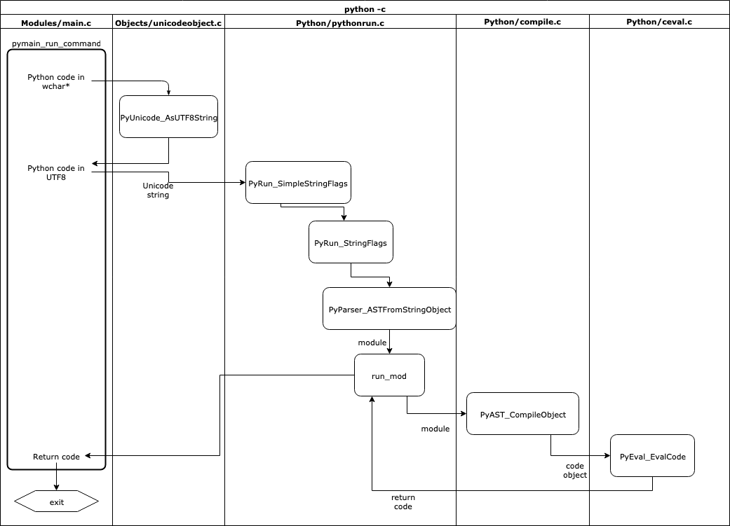
First, the pymain_run_command() function is executed inside Modules/main.c taking the command passed in -c as an argument in the C type wchar_t*. The wchar_t* type is often used as a low-level storage type for Unicode data across CPython as the size of the type can store UTF8 characters.
When converting the wchar_t* to a Python string, the Objects/unicodeobject.c file has a helper function PyUnicode_FromWideChar() that returns a PyObject, of type str. The encoding to UTF8 is then done by PyUnicode_AsUTF8String() on the Python str object to convert it to a Python bytes object.
Once this is complete, pymain_run_command() will then pass the Python bytes object to PyRun_SimpleStringFlags() for execution, but first converting the bytes to a str type again:
static int
pymain_run_command(wchar_t *command, PyCompilerFlags *cf)
{
    PyObject *unicode, *bytes;
    int ret;

    unicode = PyUnicode_FromWideChar(command, -1);
    if (unicode == NULL) {
        goto error;
    }

    if (PySys_Audit("cpython.run_command", "O", unicode) < 0) {
        return pymain_exit_err_print();
    }

    bytes = PyUnicode_AsUTF8String(unicode);
    Py_DECREF(unicode);
    if (bytes == NULL) {
        goto error;
    }

    ret = PyRun_SimpleStringFlags(PyBytes_AsString(bytes), cf);
    Py_DECREF(bytes);
    return (ret != 0);

error:
    PySys_WriteStderr("Unable to decode the command from the command line:\n");
    return pymain_exit_err_print();
}
The conversion of wchar_t* to Unicode, bytes, and then a string is roughly equivalent to the following:
unicode = str(command)
bytes_ = bytes(unicode.encode('utf8'))
# call PyRun_SimpleStringFlags with bytes_
The PyRun_SimpleStringFlags() function is part of Python/pythonrun.c. It’s purpose is to turn this simple command into a Python module and then send it on to be executed.
Since a Python module needs to have __main__ to be executed as a standalone module, it creates that automatically:
int
PyRun_SimpleStringFlags(const char *command, PyCompilerFlags *flags)
{
    PyObject *m, *d, *v;
    m = PyImport_AddModule("__main__");
    if (m == NULL)
        return -1;
    d = PyModule_GetDict(m);
    v = PyRun_StringFlags(command, Py_file_input, d, d, flags);
    if (v == NULL) {
        PyErr_Print();
        return -1;
    }
    Py_DECREF(v);
    return 0;
}
Once PyRun_SimpleStringFlags() has created a module and a dictionary, it calls PyRun_StringFlags(), which creates a fake filename and then calls the Python parser to create an AST from the string and return a module, mod:
PyObject *
PyRun_StringFlags(const char *str, int start, PyObject *globals,
                  PyObject *locals, PyCompilerFlags *flags)
{
...
    mod = PyParser_ASTFromStringObject(str, filename, start, flags, arena);
    if (mod != NULL)
        ret = run_mod(mod, filename, globals, locals, flags, arena);
    PyArena_Free(arena);
    return ret;
You’ll dive into the AST and Parser code in the next section.
-mAnother way to execute Python commands is by using the -m option with the name of a module.
A typical example is python -m unittest to run the unittest module in the standard library.
Being able to execute modules as scripts were initially proposed in PEP 338 and then the standard for explicit relative imports defined in PEP366.
The use of the -m flag implies that within the module package, you want to execute whatever is inside __main__. It also implies that you want to search sys.path for the named module.
This search mechanism is why you don’t need to remember where the unittest module is stored on your filesystem.
Inside Modules/main.c there is a function called when the command-line is run with the -m flag. The name of the module is passed as the modname argument.
CPython will then import a standard library module, runpy and execute it using PyObject_Call(). The import is done using the C API function PyImport_ImportModule(), found within the Python/import.c file:
static int
pymain_run_module(const wchar_t *modname, int set_argv0)
{
    PyObject *module, *runpy, *runmodule, *runargs, *result;
    runpy = PyImport_ImportModule("runpy");
 ...
    runmodule = PyObject_GetAttrString(runpy, "_run_module_as_main");
 ...
    module = PyUnicode_FromWideChar(modname, wcslen(modname));
 ...
    runargs = Py_BuildValue("(Oi)", module, set_argv0);
 ...
    result = PyObject_Call(runmodule, runargs, NULL);
 ...
    if (result == NULL) {
        return pymain_exit_err_print();
    }
    Py_DECREF(result);
    return 0;
}
In this function you’ll also see 2 other C API functions: PyObject_Call() and PyObject_GetAttrString(). Because PyImport_ImportModule() returns a PyObject*, the core object type, you need to call special functions to get attributes and to call it.
In Python, if you had an object and wanted to get an attribute, then you could call getattr(). In the C API, this call is PyObject_GetAttrString(), which is found in Objects/object.c. If you wanted to run a callable, you would give it parentheses, or you can run the __call__() property on any Python object. The __call__() method is implemented inside Objects/object.c:
hi = "hi!"
hi.upper() == hi.upper.__call__()  # this is the same
The runpy module is written in pure Python and located in Lib/runpy.py.
Executing python -m <module> is equivalent to running python -m runpy <module>. The runpy module was created to abstract the process of locating and executing modules on an operating system.
runpy does a few things to run the target module:
__import__() for the module name you provided__name__ (the module name) to a namespace called __main____main__ namespaceThe runpy module also supports executing directories and zip files.
If the first argument to python was a filename, such as python test.py, then CPython will open a file handle, similar to using open() in Python and pass the handle to PyRun_SimpleFileExFlags() inside Python/pythonrun.c.
There are 3 paths this function can take:
.pyc file, it will call run_pyc_file()..py) it will run PyRun_FileExFlags().stdin because the user ran command | python then treat stdin as a file handle and run PyRun_FileExFlags().int
PyRun_SimpleFileExFlags(FILE *fp, const char *filename, int closeit,
PyCompilerFlags *flags)
{
...
m = PyImport_AddModule("__main__");
...
if (maybe_pyc_file(fp, filename, ext, closeit)) {
...
v = run_pyc_file(pyc_fp, filename, d, d, flags);
} else {
/* When running from stdin, leave __main__.__loader__ alone */
if (strcmp(filename, "<stdin>") != 0 &&
set_main_loader(d, filename, "SourceFileLoader") < 0) {
fprintf(stderr, "python: failed to set __main__.__loader__\n");
ret = -1;
goto done;
}
v = PyRun_FileExFlags(fp, filename, Py_file_input, d, d,
closeit, flags);
}
...
return ret;
}
PyRun_FileExFlags()For stdin and basic script files, CPython will pass the file handle to PyRun_FileExFlags() located in the pythonrun.c file.
The purpose of PyRun_FileExFlags() is similar to PyRun_SimpleStringFlags() used for the -c input. CPython will load the file handle into PyParser_ASTFromFileObject(). We’ll cover the Parser and AST modules in the next section.
Because this is a full script, it doesn’t need the PyImport_AddModule("__main__"); step used by -c:
PyObject *
PyRun_FileExFlags(FILE *fp, const char *filename_str, int start, PyObject *globals,
                  PyObject *locals, int closeit, PyCompilerFlags *flags)
{
 ...
    mod = PyParser_ASTFromFileObject(fp, filename, NULL, start, 0, 0,
                                     flags, NULL, arena);
 ...
    ret = run_mod(mod, filename, globals, locals, flags, arena);
}
Identical to PyRun_SimpleStringFlags(), once PyRun_FileExFlags() has created a Python module from the file, it sent it to run_mod() to be executed.
run_mod() is found within Python/pythonrun.c, and sends the module to the AST to be compiled into a code object. Code objects are a format used to store the bytecode operations and the format kept in .pyc files:
static PyObject *
run_mod(mod_ty mod, PyObject *filename, PyObject *globals, PyObject *locals,
            PyCompilerFlags *flags, PyArena *arena)
{
    PyCodeObject *co;
    PyObject *v;
    co = PyAST_CompileObject(mod, filename, flags, -1, arena);
    if (co == NULL)
        return NULL;

    if (PySys_Audit("exec", "O", co) < 0) {
        Py_DECREF(co);
        return NULL;
    }

    v = run_eval_code_obj(co, globals, locals);
    Py_DECREF(co);
    return v;
}
We will cover the CPython compiler and bytecodes in the next section. The call to run_eval_code_obj() is a simple wrapper function that calls PyEval_EvalCode() in the Python/eval.c file. The PyEval_EvalCode() function is the main evaluation loop for CPython, it iterates over each bytecode statement and executes it on your local machine.
run_pyc_file()In the PyRun_SimpleFileExFlags() there was a clause for the user providing a file path to a .pyc file. If the file path ended in .pyc then instead of loading the file as a plain text file and parsing it, it will assume that the .pyc file contains a code object written to disk.
The run_pyc_file() function inside Python/pythonrun.c then marshals the code object from the .pyc file by using the file handle. Marshaling is a technical term for copying the contents of a file into memory and converting them to a specific data structure. The code object data structure on the disk is the CPython compiler’s way to caching compiled code so that it doesn’t need to parse it every time the script is called:
static PyObject *
run_pyc_file(FILE *fp, const char *filename, PyObject *globals,
             PyObject *locals, PyCompilerFlags *flags)
{
    PyCodeObject *co;
    PyObject *v;
  ...
    v = PyMarshal_ReadLastObjectFromFile(fp);
  ...
    if (v == NULL || !PyCode_Check(v)) {
        Py_XDECREF(v);
        PyErr_SetString(PyExc_RuntimeError,
                   "Bad code object in .pyc file");
        goto error;
    }
    fclose(fp);
    co = (PyCodeObject *)v;
    v = run_eval_code_obj(co, globals, locals);
    if (v && flags)
        flags->cf_flags |= (co->co_flags & PyCF_MASK);
    Py_DECREF(co);
    return v;
}
Once the code object has been marshaled to memory, it is sent to run_eval_code_obj(), which calls Python/ceval.c to execute the code.
In the exploration of reading and executing Python files, we dived as deep as the parser and AST modules, with function calls to PyParser_ASTFromFileObject().
Sticking within Python/pythonrun.c, the PyParser_ASTFromFileObject() function will take a file handle, compiler flags and a PyArena instance and convert the file object into a node object using PyParser_ParseFileObject().
With the node object, it will then convert that into a module using the AST function PyAST_FromNodeObject():
mod_ty
PyParser_ASTFromFileObject(FILE *fp, PyObject *filename, const char* enc,
                           int start, const char *ps1,
                           const char *ps2, PyCompilerFlags *flags, int *errcode,
                           PyArena *arena)
{
    ...
    node *n = PyParser_ParseFileObject(fp, filename, enc,
                                       &_PyParser_Grammar,
                                       start, ps1, ps2, &err, &iflags);
    ...
    if (n) {
        flags->cf_flags |= iflags & PyCF_MASK;
        mod = PyAST_FromNodeObject(n, flags, filename, arena);
        PyNode_Free(n);
    ...
    return mod;
}
For PyParser_ParseFileObject() we switch to Parser/parsetok.c and the parser-tokenizer stage of the CPython interpreter. This function has two important tasks:
tok_state using PyTokenizer_FromFile() in Parser/tokenizer.cnode) using parsetok() in Parser/parsetok.c node *
PyParser_ParseFileObject(FILE *fp, PyObject *filename,
const char *enc, grammar *g, int start,
const char *ps1, const char *ps2,
perrdetail *err_ret, int *flags)
{
struct tok_state *tok;
...
if ((tok = PyTokenizer_FromFile(fp, enc, ps1, ps2)) == NULL) {
err_ret->error = E_NOMEM;
return NULL;
}
...
return parsetok(tok, g, start, err_ret, flags);
}
tok_state (defined in Parser/tokenizer.h) is the data structure to store all temporary data generated by the tokenizer. It is returned to the parser-tokenizer as the data structure is required by parsetok() to develop the concrete syntax tree.
Inside parsetok(), it will use the tok_state structure and make calls to tok_get() in a loop until the file is exhausted and no more tokens can be found.
tok_get(), defined in Parser/tokenizer.c behaves like an iterator. It will keep returning the next token in the parse tree.
tok_get() is one of the most complex functions in the whole CPython codebase. It has over 640 lines and includes decades of heritage with edge cases, new language features, and syntax.
One of the simpler examples would be the part that converts a newline break into a NEWLINE token:
static int
tok_get(struct tok_state *tok, char **p_start, char **p_end)
{
...
    /* Newline */
    if (c == '\n') {
        tok->atbol = 1;
        if (blankline || tok->level > 0) {
            goto nextline;
        }
        *p_start = tok->start;
        *p_end = tok->cur - 1; /* Leave '\n' out of the string */
        tok->cont_line = 0;
        if (tok->async_def) {
            /* We're somewhere inside an 'async def' function, and
               we've encountered a NEWLINE after its signature. */
            tok->async_def_nl = 1;
        }
        return NEWLINE;
    }
...
}
In this case, NEWLINE is a token, with a value defined in Include/token.h. All tokens are constant int values, and the Include/token.h file was generated earlier when we ran make regen-grammar.
The node type returned by PyParser_ParseFileObject() is going to be essential for the next stage, converting a parse tree into an Abstract-Syntax-Tree (AST):
typedef struct _node {
    short               n_type;
    char                *n_str;
    int                 n_lineno;
    int                 n_col_offset;
    int                 n_nchildren;
    struct _node        *n_child;
    int                 n_end_lineno;
    int                 n_end_col_offset;
} node;
Since the CST is a tree of syntax, token IDs, and symbols, it would be difficult for the compiler to make quick decisions based on the Python language.
That is why the next stage is to convert the CST into an AST, a much higher-level structure. This task is performed by the Python/ast.c module, which has both a C and Python API.
Before you jump into the AST, there is a way to access the output from the parser stage. CPython has a standard library module parser, which exposes the C functions with a Python API.
The module is documented as an implementation detail of CPython so that you won’t see it in other Python interpreters. Also the output from the functions is not that easy to read.
The output will be in the numeric form, using the token and symbol numbers generated by the make regen-grammar stage, stored in Include/token.h:
>>> from pprint import pprint
>>> import parser
>>> st = parser.expr('a + 1')
>>> pprint(parser.st2list(st))
[258,
 [332,
  [306,
   [310,
    [311,
     [312,
      [313,
       [316,
        [317,
         [318,
          [319,
           [320,
            [321, [322, [323, [324, [325, [1, 'a']]]]]],
            [14, '+'],
            [321, [322, [323, [324, [325, [2, '1']]]]]]]]]]]]]]]]],
 [4, ''],
 [0, '']]
To make it easier to understand, you can take all the numbers in the symbol and token modules, put them into a dictionary and recursively replace the values in the output of parser.st2list() with the names:
import symbol
import token
import parser

def lex(expression):
    symbols = {v: k for k, v in symbol.__dict__.items() if isinstance(v, int)}
    tokens = {v: k for k, v in token.__dict__.items() if isinstance(v, int)}
    lexicon = {**symbols, **tokens}
    st = parser.expr(expression)
    st_list = parser.st2list(st)

    def replace(l: list):
        r = []
        for i in l:
            if isinstance(i, list):
                r.append(replace(i))
            else:
                if i in lexicon:
                    r.append(lexicon[i])
                else:
                    r.append(i)
        return r

    return replace(st_list)
You can run lex() with a simple expression, like a + 1 to see how this is represented as a parser-tree:
>>> from pprint import pprint
>>> pprint(lex('a + 1'))

['eval_input',
 ['testlist',
  ['test',
   ['or_test',
    ['and_test',
     ['not_test',
      ['comparison',
       ['expr',
        ['xor_expr',
         ['and_expr',
          ['shift_expr',
           ['arith_expr',
            ['term',
             ['factor', ['power', ['atom_expr', ['atom', ['NAME', 'a']]]]]],
            ['PLUS', '+'],
            ['term',
             ['factor',
              ['power', ['atom_expr', ['atom', ['NUMBER', '1']]]]]]]]]]]]]]]]],
 ['NEWLINE', ''],
 ['ENDMARKER', '']]
In the output, you can see the symbols in lowercase, such as 'test' and the tokens in uppercase, such as 'NUMBER'.
The next stage in the CPython interpreter is to convert the CST generated by the parser into something more logical that can be executed. The structure is a higher-level representation of the code, called an Abstract Syntax Tree (AST).
ASTs are produced inline with the CPython interpreter process, but you can also generate them in both Python using the ast module in the Standard Library as well as through the C API.
Before diving into the C implementation of the AST, it would be useful to understand what an AST looks like for a simple piece of Python code.
To do this, here’s a simple app called instaviz for this tutorial. It displays the AST and bytecode instructions (which we’ll cover later) in a Web UI.
To install instaviz:
$ pip install instaviz
Then, open up a REPL by running python at the command line with no arguments:
>>> import instaviz
>>> def example():
       a = 1
       b = a + 1
       return b

>>> instaviz.show(example)
You’ll see a notification on the command-line that a web server has started on port 8080. If you were using that port for something else, you can change it by calling instaviz.show(example, port=9090) or another port number.
In the web browser, you can see the detailed breakdown of your function:

The bottom left graph is the function you declared in REPL, represented as an Abstract Syntax Tree. Each node in the tree is an AST type. They are found in the ast module, and all inherit from _ast.AST.
Some of the nodes have properties which link them to child nodes, unlike the CST, which has a generic child node property.
For example, if you click on the Assign node in the center, this links to the line b = a + 1:
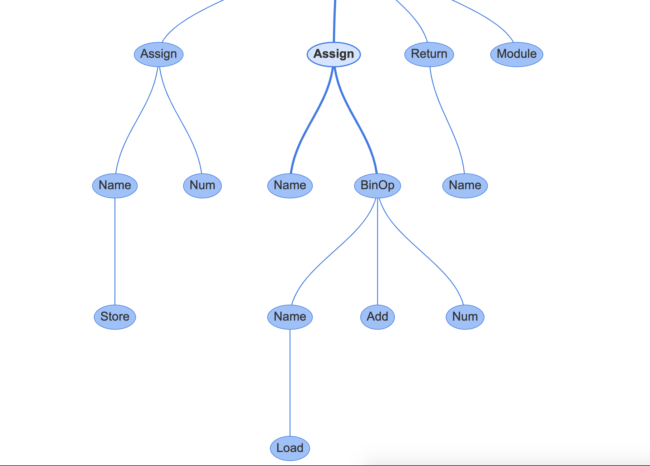
It has two properties:
targets is a list of names to assign. It is a list because you can assign to multiple variables with a single expression using unpackingvalue is the value to assign, which in this case is a BinOp statement, a + 1.If you click on the BinOp statement, it shows the properties of relevance:
left: the node to the left of the operatorop: the operator, in this case, an Add node (+) for additionright: the node to the right of the operator
Compiling an AST in C is not a straightforward task, so the Python/ast.c module is over 5000 lines of code.
There are a few entry points, forming part of the AST’s public API. In the last section on the lexer and parser, you stopped when you’d reached the call to PyAST_FromNodeObject(). By this stage, the Python interpreter process had created a CST in the format of node * tree.
Jumping then into PyAST_FromNodeObject() inside Python/ast.c, you can see it receives the node * tree, the filename, compiler flags, and the PyArena.
The return type from this function is mod_ty, defined in Include/Python-ast.h. mod_ty is a container structure for one of the 5 module types in Python:
Module InteractiveExpressionFunctionTypeSuiteIn Include/Python-ast.h you can see that an Expression type requires a field body, which is an expr_ty type. The expr_ty type is also defined in Include/Python-ast.h:
enum _mod_kind {Module_kind=1, Interactive_kind=2, Expression_kind=3,
                 FunctionType_kind=4, Suite_kind=5};
struct _mod {
    enum _mod_kind kind;
    union {
        struct {
            asdl_seq *body;
            asdl_seq *type_ignores;
        } Module;

        struct {
            asdl_seq *body;
        } Interactive;

        struct {
            expr_ty body;
        } Expression;

        struct {
            asdl_seq *argtypes;
            expr_ty returns;
        } FunctionType;

        struct {
            asdl_seq *body;
        } Suite;

    } v;
};
The AST types are all listed in Parser/Python.asdl. You will see the module types, statement types, expression types, operators, and comprehensions all listed. The names of the types in this document relate to the classes generated by the AST and the same classes named in the ast standard module library.
The parameters and names in Include/Python-ast.h correlate directly to those specified in Parser/Python.asdl:
-- ASDL's 5 builtin types are:
-- identifier, int, string, object, constant

module Python
{
    mod = Module(stmt* body, type_ignore *type_ignores)
        | Interactive(stmt* body)
        | Expression(expr body)
        | FunctionType(expr* argtypes, expr returns)
The C header file and structures are there so that the Python/ast.c program can quickly generate the structures with pointers to the relevant data.
Looking at PyAST_FromNodeObject() you can see that it is essentially a switch statement around the result from TYPE(n). TYPE() is one of the core functions used by the AST to determine what type a node in the concrete syntax tree is. In the case of PyAST_FromNodeObject() it’s just looking at the first node, so it can only be one of the module types defined as Module, Interactive, Expression, FunctionType.
The result of TYPE() will be either a symbol or token type, which we’re very familiar with by this stage.
For file_input, the results should be a Module. Modules are a series of statements, of which there are a few types. The logic to traverse the children of n and create statement nodes is within ast_for_stmt(). This function is called either once, if there is only 1 statement in the module, or in a loop if there are many. The resulting Module is then returned with the PyArena.
For eval_input, the result should be an Expression. The result from CHILD(n ,0), which is the first child of n is passed to ast_for_testlist() which returns an expr_ty type. This expr_ty is sent to Expression() with the PyArena to create an expression node, and then passed back as a result:
mod_ty
PyAST_FromNodeObject(const node *n, PyCompilerFlags *flags,
                     PyObject *filename, PyArena *arena)
{
    ...
    switch (TYPE(n)) {
        case file_input:
            stmts = _Py_asdl_seq_new(num_stmts(n), arena);
            if (!stmts)
                goto out;
            for (i = 0; i < NCH(n) - 1; i++) {
                ch = CHILD(n, i);
                if (TYPE(ch) == NEWLINE)
                    continue;
                REQ(ch, stmt);
                num = num_stmts(ch);
                if (num == 1) {
                    s = ast_for_stmt(&c, ch);
                    if (!s)
                        goto out;
                    asdl_seq_SET(stmts, k++, s);
                }
                else {
                    ch = CHILD(ch, 0);
                    REQ(ch, simple_stmt);
                    for (j = 0; j < num; j++) {
                        s = ast_for_stmt(&c, CHILD(ch, j * 2));
                        if (!s)
                            goto out;
                        asdl_seq_SET(stmts, k++, s);
                    }
                }
            }

            /* Type ignores are stored under the ENDMARKER in file_input. */
            ...

            res = Module(stmts, type_ignores, arena);
            break;
        case eval_input: {
            expr_ty testlist_ast;

            /* XXX Why not comp_for here? */
            testlist_ast = ast_for_testlist(&c, CHILD(n, 0));
            if (!testlist_ast)
                goto out;
            res = Expression(testlist_ast, arena);
            break;
        }
        case single_input:
            ...
            break;
        case func_type_input:
            ...
        ...
    return res;
}
Inside the ast_for_stmt() function, there is another switch statement for each possible statement type (simple_stmt, compound_stmt, and so on) and the code to determine the arguments to the node class.
One of the simpler functions is for the power expression, i.e., 2**4 is 2 to the power of 4. This function starts by getting the ast_for_atom_expr(), which is the number 2 in our example, then if that has one child, it returns the atomic expression. If it has more than one child, it will get the right-hand (the number 4) and return a BinOp (binary operation) with the operator as Pow (power), the left hand of e (2), and the right hand of f (4):
static expr_ty
ast_for_power(struct compiling *c, const node *n)
{
    /* power: atom trailer* ('**' factor)*
     */
    expr_ty e;
    REQ(n, power);
    e = ast_for_atom_expr(c, CHILD(n, 0));
    if (!e)
        return NULL;
    if (NCH(n) == 1)
        return e;
    if (TYPE(CHILD(n, NCH(n) - 1)) == factor) {
        expr_ty f = ast_for_expr(c, CHILD(n, NCH(n) - 1));
        if (!f)
            return NULL;
        e = BinOp(e, Pow, f, LINENO(n), n->n_col_offset,
                  n->n_end_lineno, n->n_end_col_offset, c->c_arena);
    }
    return e;
}
You can see the result of this if you send a short function to the instaviz module:
>>> def foo():
       2**4
>>> import instaviz
>>> instaviz.show(foo)

In the UI you can also see the corresponding properties:

In summary, each statement type and expression has a corresponding ast_for_*() function to create it. The arguments are defined in Parser/Python.asdl and exposed via the ast module in the standard library. If an expression or statement has children, then it will call the corresponding ast_for_* child function in a depth-first traversal.
CPython’s versatility and low-level execution API make it the ideal candidate for an embedded scripting engine. You will see CPython used in many UI applications, such as Game Design, 3D graphics and system automation.
The interpreter process is flexible and efficient, and now you have an understanding of how it works you’re ready to understand the compiler.
In Part 2, you saw how the CPython interpreter takes an input, such as a file or string, and converts it into a logical Abstract Syntax Tree. We’re still not at the stage where this code can be executed. Next, we have to go deeper to convert the Abstract Syntax Tree into a set of sequential commands that the CPU can understand.
Now the interpreter has an AST with the properties required for each of the operations, functions, classes, and namespaces. It is the job of the compiler to turn the AST into something the CPU can understand.
This compilation task is split into 2 parts:
Earlier, we were looking at how files are executed, and the PyRun_FileExFlags() function in Python/pythonrun.c. Inside this function, we converted the FILE handle into a mod, of type mod_ty. This task was completed by PyParser_ASTFromFileObject(), which in turns calls the tokenizer, parser-tokenizer and then the AST:
PyObject *
PyRun_FileExFlags(FILE *fp, const char *filename_str, int start, PyObject *globals,
                  PyObject *locals, int closeit, PyCompilerFlags *flags)
{
 ...
    mod = PyParser_ASTFromFileObject(fp, filename, NULL, start, 0, 0,
 ...
    ret = run_mod(mod, filename, globals, locals, flags, arena);
}
The resulting module from the call to is sent to run_mod() still in Python/pythonrun.c. This is a small function that gets a PyCodeObject from PyAST_CompileObject() and sends it on to run_eval_code_obj(). You will tackle run_eval_code_obj() in the next section:
static PyObject *
run_mod(mod_ty mod, PyObject *filename, PyObject *globals, PyObject *locals,
            PyCompilerFlags *flags, PyArena *arena)
{
    PyCodeObject *co;
    PyObject *v;
    co = PyAST_CompileObject(mod, filename, flags, -1, arena);
    if (co == NULL)
        return NULL;

    if (PySys_Audit("exec", "O", co) < 0) {
        Py_DECREF(co);
        return NULL;
    }

    v = run_eval_code_obj(co, globals, locals);
    Py_DECREF(co);
    return v;
}
The PyAST_CompileObject() function is the main entry point to the CPython compiler. It takes a Python module as its primary argument, along with the name of the file, the globals, locals, and the PyArena all created earlier in the interpreter process.
We’re starting to get into the guts of the CPython compiler now, with decades of development and Computer Science theory behind it. Don’t be put off by the language. Once we break down the compiler into logical steps, it’ll make sense.
Before the compiler starts, a global compiler state is created. This type, compiler is defined in Python/compile.c and contains properties used by the compiler to remember the compiler flags, the stack, and the PyArena:
struct compiler {
    PyObject *c_filename;
    struct symtable *c_st;
    PyFutureFeatures *c_future; /* pointer to module's __future__ */
    PyCompilerFlags *c_flags;

    int c_optimize;              /* optimization level */
    int c_interactive;           /* true if in interactive mode */
    int c_nestlevel;
    int c_do_not_emit_bytecode;  /* The compiler won't emit any bytecode
                                    if this value is different from zero.
                                    This can be used to temporarily visit
                                    nodes without emitting bytecode to
                                    check only errors. */

    PyObject *c_const_cache;     /* Python dict holding all constants,
                                    including names tuple */
    struct compiler_unit *u; /* compiler state for current block */
    PyObject *c_stack;           /* Python list holding compiler_unit ptrs */
    PyArena *c_arena;            /* pointer to memory allocation arena */
};
Inside PyAST_CompileObject(), there are 11 main steps happening:
__doc__ property to the module if it doesn’t exist.__annotations__ property to the module if it doesn’t exist.__future__ flags in the module to the future flags in the compiler.__future__ features in the compiler.PyCodeObject *
PyAST_CompileObject(mod_ty mod, PyObject *filename, PyCompilerFlags *flags,
int optimize, PyArena *arena)
{
struct compiler c;
PyCodeObject *co = NULL;
PyCompilerFlags local_flags = _PyCompilerFlags_INIT;
int merged;
PyConfig *config = &_PyInterpreterState_GET_UNSAFE()->config;
if (!__doc__) {
__doc__ = PyUnicode_InternFromString("__doc__");
if (!__doc__)
return NULL;
}
if (!__annotations__) {
__annotations__ = PyUnicode_InternFromString("__annotations__");
if (!__annotations__)
return NULL;
}
if (!compiler_init(&c))
return NULL;
Py_INCREF(filename);
c.c_filename = filename;
c.c_arena = arena;
c.c_future = PyFuture_FromASTObject(mod, filename);
if (c.c_future == NULL)
goto finally;
if (!flags) {
flags = &local_flags;
}
merged = c.c_future->ff_features | flags->cf_flags;
c.c_future->ff_features = merged;
flags->cf_flags = merged;
c.c_flags = flags;
c.c_optimize = (optimize == -1) ? config->optimization_level : optimize;
c.c_nestlevel = 0;
c.c_do_not_emit_bytecode = 0;
if (!_PyAST_Optimize(mod, arena, c.c_optimize)) {
goto finally;
}
c.c_st = PySymtable_BuildObject(mod, filename, c.c_future);
if (c.c_st == NULL) {
if (!PyErr_Occurred())
PyErr_SetString(PyExc_SystemError, "no symtable");
goto finally;
}
co = compiler_mod(&c, mod);
finally:
compiler_free(&c);
assert(co || PyErr_Occurred());
return co;
}
Before the compiler runs, there are two types of flags to toggle the features inside the compiler. These come from two places:
pyconfig.h or via environment variables__future__ statements inside the actual source code of the moduleTo distinguish the two types of flags, think that the __future__ flags are required because of the syntax or features in that specific module. For example, Python 3.7 introduced delayed evaluation of type hints through the annotations future flag:
from __future__ import annotations
The code after this statement might use unresolved type hints, so the __future__ statement is required. Otherwise, the module wouldn’t import. It would be unmaintainable to manually request that the person importing the module enable this specific compiler flag.
The other compiler flags are specific to the environment, so they might change the way the code executes or the way the compiler runs, but they shouldn’t link to the source in the same way that __future__ statements do.
One example of a compiler flag would be the -O flag for optimizing the use of assert statements. This flag disables any assert statements, which may have been put in the code for debugging purposes.
It can also be enabled with the PYTHONOPTIMIZE=1 environment variable setting.
In PyAST_CompileObject() there was a reference to a symtable and a call to PySymtable_BuildObject() with the module to be executed.
The purpose of the symbol table is to provide a list of namespaces, globals, and locals for the compiler to use for referencing and resolving scopes.
The symtable structure in Include/symtable.h is well documented, so it’s clear what each of the fields is for. There should be one symtable instance for the compiler, so namespacing becomes essential.
If you create a function called resolve_names() in one module and declare another function with the same name in another module, you want to be sure which one is called. The symtable serves this purpose, as well as ensuring that variables declared within a narrow scope don’t automatically become globals (after all, this isn’t JavaScript):
struct symtable {
    PyObject *st_filename;          /* name of file being compiled,
                                       decoded from the filesystem encoding */
    struct _symtable_entry *st_cur; /* current symbol table entry */
    struct _symtable_entry *st_top; /* symbol table entry for module */
    PyObject *st_blocks;            /* dict: map AST node addresses
                                     *       to symbol table entries */
    PyObject *st_stack;             /* list: stack of namespace info */
    PyObject *st_global;            /* borrowed ref to st_top->ste_symbols */
    int st_nblocks;                 /* number of blocks used. kept for
                                       consistency with the corresponding
                                       compiler structure */
    PyObject *st_private;           /* name of current class or NULL */
    PyFutureFeatures *st_future;    /* module's future features that affect
                                       the symbol table */
    int recursion_depth;            /* current recursion depth */
    int recursion_limit;            /* recursion limit */
};
Some of the symbol table API is exposed via the symtable module in the standard library. You can provide an expression or a module an receive a symtable.SymbolTable instance.
You can provide a string with a Python expression and the compile_type of "eval", or a module, function or class, and the compile_mode of "exec" to get a symbol table.
Looping over the elements in the table we can see some of the public and private fields and their types:
>>> import symtable
>>> s = symtable.symtable('b + 1', filename='test.py', compile_type='eval')
>>> [symbol.__dict__ for symbol in s.get_symbols()]
[{'_Symbol__name': 'b', '_Symbol__flags': 6160, '_Symbol__scope': 3, '_Symbol__namespaces': ()}]
The C code behind this is all within Python/symtable.c and the primary interface is the PySymtable_BuildObject() function.
Similar to the top-level AST function we covered earlier, the PySymtable_BuildObject() function switches between the mod_ty possible types (Module, Expression, Interactive, Suite, FunctionType), and visits each of the statements inside them.
Remember, mod_ty is an AST instance, so the will now recursively explore the nodes and branches of the tree and add entries to the symtable:
struct symtable *
PySymtable_BuildObject(mod_ty mod, PyObject *filename, PyFutureFeatures *future)
{
    struct symtable *st = symtable_new();
    asdl_seq *seq;
    int i;
    PyThreadState *tstate;
    int recursion_limit = Py_GetRecursionLimit();
...
    st->st_top = st->st_cur;
    switch (mod->kind) {
    case Module_kind:
        seq = mod->v.Module.body;
        for (i = 0; i < asdl_seq_LEN(seq); i++)
            if (!symtable_visit_stmt(st,
                        (stmt_ty)asdl_seq_GET(seq, i)))
                goto error;
        break;
    case Expression_kind:
        ...
    case Interactive_kind:
        ...
    case Suite_kind:
        ...
    case FunctionType_kind:
        ...
    }
    ...
}
So for a module, PySymtable_BuildObject() will loop through each statement in the module and call symtable_visit_stmt(). The symtable_visit_stmt() is a huge switch statement with a case for each statement type (defined in Parser/Python.asdl).
For each statement type, there is specific logic to that statement type. For example, a function definition has particular logic for:
symtable_enter_block()Note: If you’ve ever wondered why Python’s default arguments are mutable, the reason is in this function. You can see they are a pointer to the variable in the symtable. No extra work is done to copy any values to an immutable type.
static int
symtable_visit_stmt(struct symtable *st, stmt_ty s)
{
    if (++st->recursion_depth > st->recursion_limit) {                          // 1.
        PyErr_SetString(PyExc_RecursionError,
                        "maximum recursion depth exceeded during compilation");
        VISIT_QUIT(st, 0);
    }
    switch (s->kind) {
    case FunctionDef_kind:
        if (!symtable_add_def(st, s->v.FunctionDef.name, DEF_LOCAL))            // 2.
            VISIT_QUIT(st, 0);
        if (s->v.FunctionDef.args->defaults)                                    // 3.
            VISIT_SEQ(st, expr, s->v.FunctionDef.args->defaults);
        if (s->v.FunctionDef.args->kw_defaults)                                 // 4.
            VISIT_SEQ_WITH_NULL(st, expr, s->v.FunctionDef.args->kw_defaults);
        if (!symtable_visit_annotations(st, s, s->v.FunctionDef.args,           // 5.
                                        s->v.FunctionDef.returns))
            VISIT_QUIT(st, 0);
        if (s->v.FunctionDef.decorator_list)                                    // 6.
            VISIT_SEQ(st, expr, s->v.FunctionDef.decorator_list);
        if (!symtable_enter_block(st, s->v.FunctionDef.name,                    // 7.
                                  FunctionBlock, (void *)s, s->lineno,
                                  s->col_offset))
            VISIT_QUIT(st, 0);
        VISIT(st, arguments, s->v.FunctionDef.args);                            // 8.
        VISIT_SEQ(st, stmt, s->v.FunctionDef.body);                             // 9.
        if (!symtable_exit_block(st, s))
            VISIT_QUIT(st, 0);
        break;
    case ClassDef_kind: {
        ...
    }
    case Return_kind:
        ...
    case Delete_kind:
        ...
    case Assign_kind:
        ...
    case AnnAssign_kind:
        ...
Once the resulting symtable has been created, it is sent back to be used for the compiler.
Now that the PyAST_CompileObject() has a compiler state, a symtable, and a module in the form of the AST, the actual compilation can begin.
The purpose of the core compiler is to:
You can call the CPython compiler in Python code by calling the built-in function compile(). It returns a code object instance:
>>> compile('b+1', 'test.py', mode='eval')
<code object <module> at 0x10f222780, file "test.py", line 1>
The same as with the symtable() function, a simple expression should have a mode of 'eval' and a module, function, or class should have a mode of 'exec'.
The compiled code can be found in the co_code property of the code object:
>>> co.co_code
b'e\x00d\x00\x17\x00S\x00'
There is also a dis module in the standard library, which disassembles the bytecode instructions and can print them on the screen or give you a list of Instruction instances.
If you import dis and give the dis() function the code object’s co_code property it disassembles it and prints the instructions on the REPL:
>>> import dis
>>> dis.dis(co.co_code)
          0 LOAD_NAME                0 (0)
          2 LOAD_CONST               0 (0)
          4 BINARY_ADD
          6 RETURN_VALUE
LOAD_NAME, LOAD_CONST, BINARY_ADD, and RETURN_VALUE are all bytecode instructions. They’re called bytecode because, in binary form, they were a byte long. However, since Python 3.6 the storage format was changed to a word, so now they’re technically wordcode, not bytecode.
The full list of bytecode instructions is available for each version of Python, and it does change between versions. For example, in Python 3.7, some new bytecode instructions were introduced to speed up execution of specific method calls.
In an earlier section, we explored the instaviz package. This included a visualization of the code object type by running the compiler. It also displays the Bytecode operations inside the code objects.
Execute instaviz again to see the code object and bytecode for a function defined on the REPL:
>>> import instaviz
>>> def example():
       a = 1
       b = a + 1
       return b
>>> instaviz.show(example)
If we now jump into compiler_mod(), a function used to switch to different compiler functions depending on the module type. We’ll assume that mod is a Module. The module is compiled into the compiler state and then assemble() is run to create a PyCodeObject.
The new code object is returned back to PyAST_CompileObject() and sent on for execution:
static PyCodeObject *
compiler_mod(struct compiler *c, mod_ty mod)
{
    PyCodeObject *co;
    int addNone = 1;
    static PyObject *module;
    ...
    switch (mod->kind) {
    case Module_kind:
        if (!compiler_body(c, mod->v.Module.body)) {
            compiler_exit_scope(c);
            return 0;
        }
        break;
    case Interactive_kind:
        ...
    case Expression_kind:
        ...
    case Suite_kind:
        ...
    ...
    co = assemble(c, addNone);
    compiler_exit_scope(c);
    return co;
}
The compiler_body() function has some optimization flags and then loops over each statement in the module and visits it, similar to how the symtable functions worked:
static int
compiler_body(struct compiler *c, asdl_seq *stmts)
{
    int i = 0;
    stmt_ty st;
    PyObject *docstring;
    ...
    for (; i < asdl_seq_LEN(stmts); i++)
        VISIT(c, stmt, (stmt_ty)asdl_seq_GET(stmts, i));
    return 1;
}
The statement type is determined through a call to the asdl_seq_GET() function, which looks at the AST node’s type.
Through some smart macros, VISIT calls a function in Python/compile.c for each statement type:
#define VISIT(C, TYPE, V) {\
    if (!compiler_visit_ ## TYPE((C), (V))) \
        return 0; \
}
For a stmt (the category for a statement) the compiler will then drop into compiler_visit_stmt() and switch through all of the potential statement types found in Parser/Python.asdl:
static int
compiler_visit_stmt(struct compiler *c, stmt_ty s)
{
    Py_ssize_t i, n;

    /* Always assign a lineno to the next instruction for a stmt. */
    c->u->u_lineno = s->lineno;
    c->u->u_col_offset = s->col_offset;
    c->u->u_lineno_set = 0;

    switch (s->kind) {
    case FunctionDef_kind:
        return compiler_function(c, s, 0);
    case ClassDef_kind:
        return compiler_class(c, s);
    ...
    case For_kind:
        return compiler_for(c, s);
    ...
    }

    return 1;
}
As an example, let’s focus on the For statement, in Python is the:
for i in iterable:
    # block
else:  # optional if iterable is False
    # block
If the statement is a For type, it calls compiler_for(). There is an equivalent compiler_*() function for all of the statement and expression types. The more straightforward types create the bytecode instructions inline, some of the more complex statement types call other functions.
Many of the statements can have sub-statements. A for loop has a body, but you can also have complex expressions in the assignment and the iterator.
The compiler’s compiler_ statements sends blocks to the compiler state. These blocks contain instructions, the instruction data structure in Python/compile.c has the opcode, any arguments, and the target block (if this is a jump instruction), it also contains the line number.
For jump statements, they can either be absolute or relative jump statements. Jump statements are used to “jump” from one operation to another. Absolute jump statements specify the exact operation number in the compiled code object, whereas relative jump statements specify the jump target relative to another operation:
struct instr {
    unsigned i_jabs : 1;
    unsigned i_jrel : 1;
    unsigned char i_opcode;
    int i_oparg;
    struct basicblock_ *i_target; /* target block (if jump instruction) */
    int i_lineno;
};
So a frame block (of type basicblock), contains the following fields:
b_list pointer, the link to a list of blocks for the compiler stateb_instr, with both the allocated list size b_ialloc, and the number used b_iusedb_nextRETURN_VALUE opcode (b_return)b_startdepth)typedef struct basicblock_ {
/* Each basicblock in a compilation unit is linked via b_list in the
reverse order that the block are allocated. b_list points to the next
block, not to be confused with b_next, which is next by control flow. */
struct basicblock_ *b_list;
/* number of instructions used */
int b_iused;
/* length of instruction array (b_instr) */
int b_ialloc;
/* pointer to an array of instructions, initially NULL */
struct instr *b_instr;
/* If b_next is non-NULL, it is a pointer to the next
block reached by normal control flow. */
struct basicblock_ *b_next;
/* b_seen is used to perform a DFS of basicblocks. */
unsigned b_seen : 1;
/* b_return is true if a RETURN_VALUE opcode is inserted. */
unsigned b_return : 1;
/* depth of stack upon entry of block, computed by stackdepth() */
int b_startdepth;
/* instruction offset for block, computed by assemble_jump_offsets() */
int b_offset;
} basicblock;
The For statement is somewhere in the middle in terms of complexity. There are 15 steps in the compilation of a For statement with the for <target> in <iterator>: syntax:
start, this allocates memory and creates a basicblock pointercleanupendFOR_LOOP to the stack with start as the entry block and end as the exit blockGET_ITER operation to the compiler statestart blockADDOP_JREL which calls compiler_addop_j() to add the FOR_ITER operation with an argument of the cleanup blocktarget and add any special code, like tuple unpacking, to the start blockADDOP_JABS which calls compiler_addop_j() to add the JUMP_ABSOLUTE operation which indicates after the body is executed, jumps back to the start of the loopcleanup blockFOR_LOOP frame block off the stackelse section of the for loopend blockReferring back to the basicblock structure. You can see how in the compilation of the for statement, the various blocks are created and pushed into the compiler’s frame block and stack:
static int
compiler_for(struct compiler *c, stmt_ty s)
{
    basicblock *start, *cleanup, *end;

    start = compiler_new_block(c);                       // 1.
    cleanup = compiler_new_block(c);                     // 2.
    end = compiler_new_block(c);                         // 3.
    if (start == NULL || end == NULL || cleanup == NULL)
        return 0;

    if (!compiler_push_fblock(c, FOR_LOOP, start, end))  // 4.
        return 0;

    VISIT(c, expr, s->v.For.iter);                       // 5.
    ADDOP(c, GET_ITER);                                  // 6.
    compiler_use_next_block(c, start);                   // 7.
    ADDOP_JREL(c, FOR_ITER, cleanup);                    // 8.
    VISIT(c, expr, s->v.For.target);                     // 9.
    VISIT_SEQ(c, stmt, s->v.For.body);                   // 10.
    ADDOP_JABS(c, JUMP_ABSOLUTE, start);                 // 11.
    compiler_use_next_block(c, cleanup);                 // 12.

    compiler_pop_fblock(c, FOR_LOOP, start);             // 13.

    VISIT_SEQ(c, stmt, s->v.For.orelse);                 // 14.
    compiler_use_next_block(c, end);                     // 15.
    return 1;
}
Depending on the type of operation, there are different arguments required. For example, we used ADDOP_JABS and ADDOP_JREL here, which refer to “ADD Operation with Jump to a RELative position” and “ADD Operation with Jump to an ABSolute position”. This is referring to the APPOP_JREL and ADDOP_JABS macros which call compiler_addop_j(struct compiler *c, int opcode, basicblock *b, int absolute) and set the absolute argument to 0 and 1 respectively.
There are some other macros, like ADDOP_I calls compiler_addop_i() which add an operation with an integer argument, or ADDOP_O calls compiler_addop_o() which adds an operation with a PyObject argument.
Once these stages have completed, the compiler has a list of frame blocks, each containing a list of instructions and a pointer to the next block.
With the compiler state, the assembler performs a “depth-first-search” of the blocks and merge the instructions into a single bytecode sequence. The assembler state is declared in Python/compile.c:
struct assembler {
    PyObject *a_bytecode;  /* string containing bytecode */
    int a_offset;              /* offset into bytecode */
    int a_nblocks;             /* number of reachable blocks */
    basicblock **a_postorder; /* list of blocks in dfs postorder */
    PyObject *a_lnotab;    /* string containing lnotab */
    int a_lnotab_off;      /* offset into lnotab */
    int a_lineno;              /* last lineno of emitted instruction */
    int a_lineno_off;      /* bytecode offset of last lineno */
};
The assemble() function has a few tasks:
None, this is why every function returns None, whether or not a return statement existsdfs() to perform a depth-first-search of the blocksmakecode() with the compiler state to generate the PyCodeObjectstatic PyCodeObject *
assemble(struct compiler *c, int addNone)
{
basicblock *b, *entryblock;
struct assembler a;
int i, j, nblocks;
PyCodeObject *co = NULL;
/* Make sure every block that falls off the end returns None.
XXX NEXT_BLOCK() isn't quite right, because if the last
block ends with a jump or return b_next shouldn't set.
*/
if (!c->u->u_curblock->b_return) {
NEXT_BLOCK(c);
if (addNone)
ADDOP_LOAD_CONST(c, Py_None);
ADDOP(c, RETURN_VALUE);
}
...
dfs(c, entryblock, &a, nblocks);
/* Can't modify the bytecode after computing jump offsets. */
assemble_jump_offsets(&a, c);
/* Emit code in reverse postorder from dfs. */
for (i = a.a_nblocks - 1; i >= 0; i--) {
b = a.a_postorder[i];
for (j = 0; j < b->b_iused; j++)
if (!assemble_emit(&a, &b->b_instr[j]))
goto error;
}
...
co = makecode(c, &a);
error:
assemble_free(&a);
return co;
}
The depth-first-search is performed by the dfs() function in Python/compile.c, which follows the the b_next pointers in each of the blocks, marks them as seen by toggling b_seen and then adds them to the assemblers **a_postorder list in reverse order.
The function loops back over the assembler’s post-order list and for each block, if it has a jump operation, recursively call dfs() for that jump:
static void
dfs(struct compiler *c, basicblock *b, struct assembler *a, int end)
{
int i, j;
/* Get rid of recursion for normal control flow.
Since the number of blocks is limited, unused space in a_postorder
(from a_nblocks to end) can be used as a stack for still not ordered
blocks. */
for (j = end; b && !b->b_seen; b = b->b_next) {
b->b_seen = 1;
assert(a->a_nblocks < j);
a->a_postorder[--j] = b;
}
while (j < end) {
b = a->a_postorder[j++];
for (i = 0; i < b->b_iused; i++) {
struct instr *instr = &b->b_instr[i];
if (instr->i_jrel || instr->i_jabs)
dfs(c, instr->i_target, a, j);
}
assert(a->a_nblocks < j);
a->a_postorder[a->a_nblocks++] = b;
}
}
The task of makecode() is to go through the compiler state, some of the assembler’s properties and to put these into a PyCodeObject by calling PyCode_New():

The variable names, constants are put as properties to the code object:
static PyCodeObject *
makecode(struct compiler *c, struct assembler *a)
{
...
consts = consts_dict_keys_inorder(c->u->u_consts);
names = dict_keys_inorder(c->u->u_names, 0);
varnames = dict_keys_inorder(c->u->u_varnames, 0);
...
cellvars = dict_keys_inorder(c->u->u_cellvars, 0);
...
freevars = dict_keys_inorder(c->u->u_freevars, PyTuple_GET_SIZE(cellvars));
...
flags = compute_code_flags(c);
if (flags < 0)
goto error;
bytecode = PyCode_Optimize(a->a_bytecode, consts, names, a->a_lnotab);
...
co = PyCode_NewWithPosOnlyArgs(posonlyargcount+posorkeywordargcount,
posonlyargcount, kwonlyargcount, nlocals_int,
maxdepth, flags, bytecode, consts, names,
varnames, freevars, cellvars, c->c_filename,
c->u->u_name, c->u->u_firstlineno, a->a_lnotab);
...
return co;
}
You may also notice that the bytecode is sent to PyCode_Optimize() before it is sent to PyCode_NewWithPosOnlyArgs(). This function is part of the bytecode optimization process in Python/peephole.c.
The peephole optimizer goes through the bytecode instructions and in certain scenarios, replace them with other instructions. For example, there is an optimizer called “constant unfolding”, so if you put the following statement into your script:
a = 1 + 5
It optimizes that to:
a = 6
Because 1 and 5 are constant values, so the result should always be the same.
We can pull together all of these stages with the instaviz module:
import instaviz
def foo():
a = 2**4
b = 1 + 5
c = [1, 4, 6]
for i in c:
print(i)
else:
print(a)
return c
instaviz.show(foo)
Will produce an AST graph:
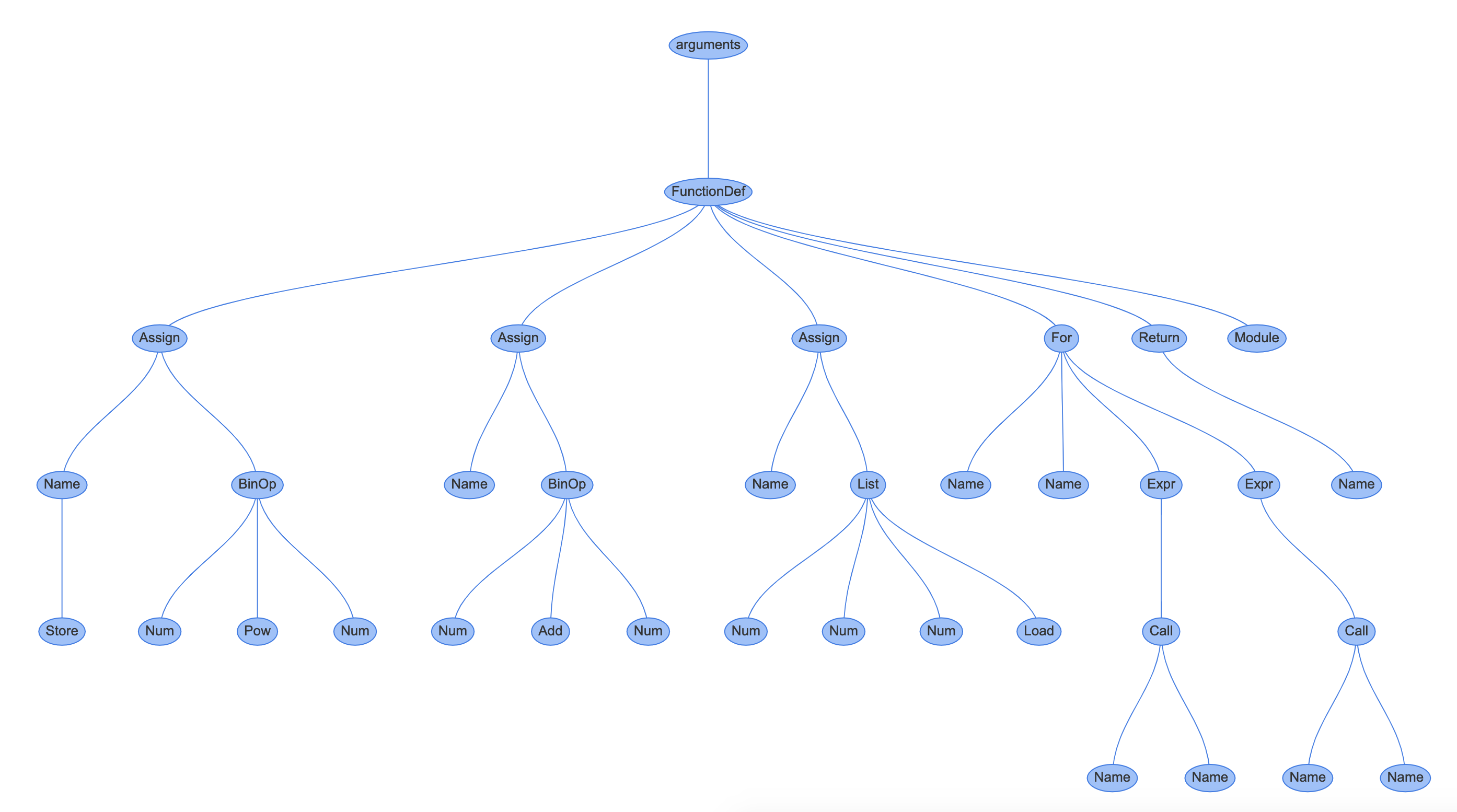
With bytecode instructions in sequence:

Also, the code object with the variable names, constants, and binary co_code:
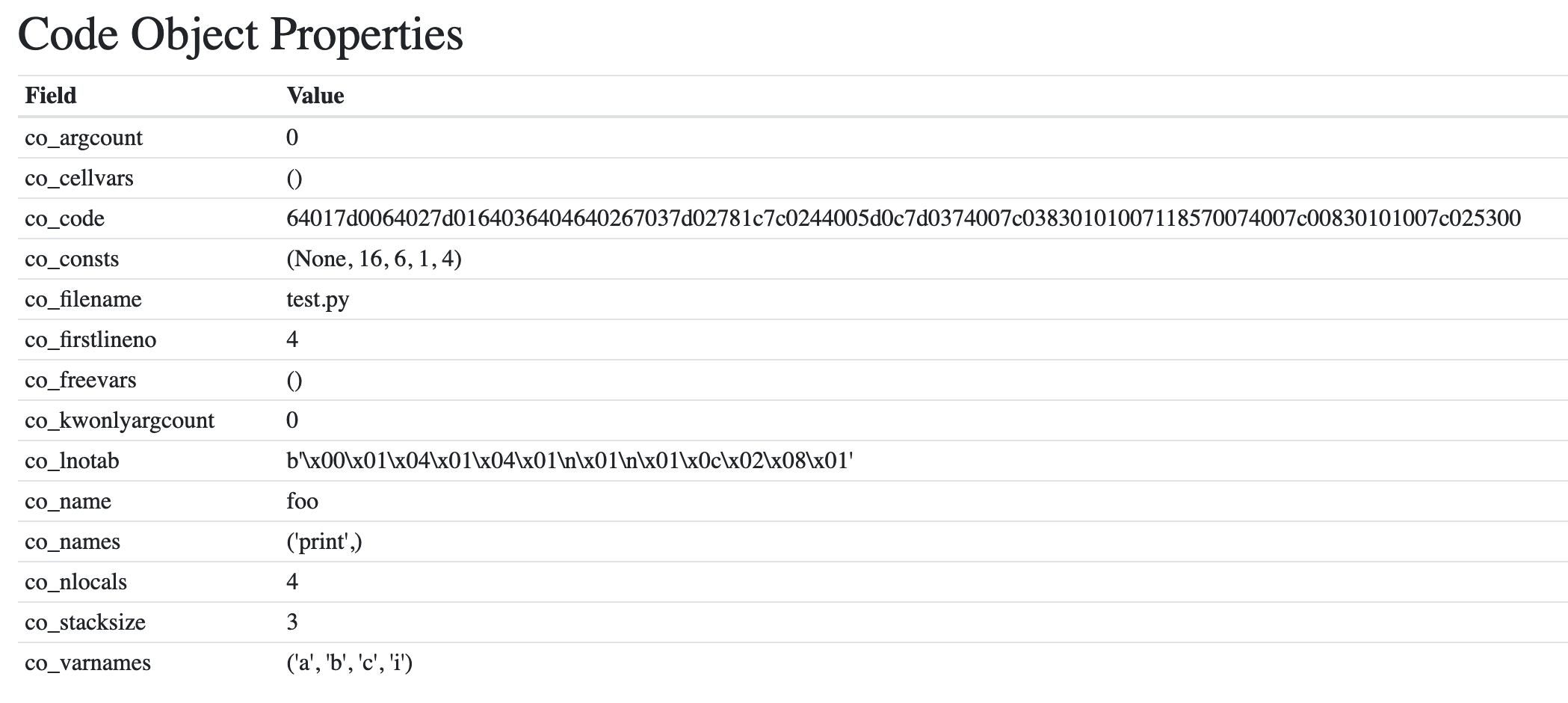
In Python/pythonrun.c we broke out just before the call to run_eval_code_obj().
This call takes a code object, either fetched from the marshaled .pyc file, or compiled through the AST and compiler stages.
run_eval_code_obj() will pass the globals, locals, PyArena, and compiled PyCodeObject to PyEval_EvalCode() in Python/ceval.c.
This stage forms the execution component of CPython. Each of the bytecode operations is taken and executed using a “Stack Frame” based system.
What is a Stack Frame?
Stack Frames are a data type used by many runtimes, not just Python, that allows functions to be called and variables to be returned between functions. Stack Frames also contain arguments, local variables, and other state information.
Typically, a Stack Frame exists for every function call, and they are stacked in sequence. You can see CPython’s frame stack anytime an exception is unhandled and the stack is printed on the screen.
PyEval_EvalCode() is the public API for evaluating a code object. The logic for evaluation is split between _PyEval_EvalCodeWithName() and _PyEval_EvalFrameDefault(), which are both in ceval.c.
The public API PyEval_EvalCode() will construct an execution frame from the top of the stack by calling _PyEval_EvalCodeWithName().
The construction of the first execution frame has many steps:
*args and **kwargs in function definitions are resolved.The frame object looks like this:

Let’s step through those sequences.
Before a frame can be executed, it needs to be referenced from a thread. CPython can have many threads running at any one time within a single interpreter. An Interpreter state includes a list of those threads as a linked list. The thread structure is called PyThreadState, and there are many references throughout ceval.c.
Here is the structure of the thread state object:
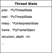
The input to PyEval_EvalCode() and therefore _PyEval_EvalCodeWithName() has arguments for:
_co: a PyCodeObjectglobals: a PyDict with variable names as keys and their valueslocals: a PyDict with variable names as keys and their valuesThe other arguments are optional, and not used for the basic API:
args: a PyTuple with positional argument values in order, and argcount for the number of valueskwnames: a list of keyword argument nameskwargs: a list of keyword argument values, and kwcount for the number of themdefs: a list of default values for positional arguments, and defcount for the lengthkwdefs: a dictionary with the default values for keyword argumentsclosure: a tuple with strings to merge into the code objects co_freevars fieldname: the name for this evaluation statement as a stringqualname: the qualified name for this evaluation statement as a stringPyObject *
_PyEval_EvalCodeWithName(PyObject *_co, PyObject *globals, PyObject *locals,
PyObject *const *args, Py_ssize_t argcount,
PyObject *const *kwnames, PyObject *const *kwargs,
Py_ssize_t kwcount, int kwstep,
PyObject *const *defs, Py_ssize_t defcount,
PyObject *kwdefs, PyObject *closure,
PyObject *name, PyObject *qualname)
{
...
PyThreadState *tstate = _PyThreadState_GET();
assert(tstate != NULL);
if (globals == NULL) {
_PyErr_SetString(tstate, PyExc_SystemError,
"PyEval_EvalCodeEx: NULL globals");
return NULL;
}
/* Create the frame */
f = _PyFrame_New_NoTrack(tstate, co, globals, locals);
if (f == NULL) {
return NULL;
}
fastlocals = f->f_localsplus;
freevars = f->f_localsplus + co->co_nlocals;
If the function definition contained a **kwargs style catch-all for keyword arguments, then a new dictionary is created, and the values are copied across. The kwargs name is then set as a variable, like in this example:
def example(arg, arg2=None, **kwargs):
print(kwargs['extra']) # this would resolve to a dictionary key
The logic for creating a keyword argument dictionary is in the next part of _PyEval_EvalCodeWithName():
/* Create a dictionary for keyword parameters (**kwargs) */
if (co->co_flags & CO_VARKEYWORDS) {
kwdict = PyDict_New();
if (kwdict == NULL)
goto fail;
i = total_args;
if (co->co_flags & CO_VARARGS) {
i++;
}
SETLOCAL(i, kwdict);
}
else {
kwdict = NULL;
}
The kwdict variable will reference a PyDictObject if any keyword arguments were found.
Next, each of the positional arguments (if provided) are set as local variables:
/* Copy all positional arguments into local variables */
if (argcount > co->co_argcount) {
n = co->co_argcount;
}
else {
n = argcount;
}
for (j = 0; j < n; j++) {
x = args[j];
Py_INCREF(x);
SETLOCAL(j, x);
}
At the end of the loop, you’ll see a call to SETLOCAL() with the value, so if a positional argument is defined with a value, that is available within this scope:
def example(arg1, arg2):
print(arg1, arg2) # both args are already local variables.
Also, the reference counter for those variables is incremented, so the garbage collector won’t remove them until the frame has evaluated.
*argsSimilar to **kwargs, a function argument prepended with a * can be set to catch all remaining positional arguments. This argument is a tuple and the *args name is set as a local variable:
/* Pack other positional arguments into the *args argument */
if (co->co_flags & CO_VARARGS) {
u = _PyTuple_FromArray(args + n, argcount - n);
if (u == NULL) {
goto fail;
}
SETLOCAL(total_args, u);
}
If the function was called with keyword arguments and values, the kwdict dictionary created in step 4 is now filled with any remaining keyword arguments passed by the caller that doesn’t resolve to named arguments or positional arguments.
For example, the e argument was neither positional or named, so it is added to **remaining:
>>> def my_function(a, b, c=None, d=None, **remaining):
print(a, b, c, d, remaining)
>>> my_function(a=1, b=2, c=3, d=4, e=5)
(1, 2, 3, 4, {'e': 5})
Positional-only arguments is a new feature in Python 3.8. Introduced in PEP570, positional-only arguments are a way of stopping users of your API from using positional arguments with a keyword syntax.
For example, this simple function converts Farenheit to Celcius. Note, the use of / as a special argument seperates positional-only arguments from the other arguments.
def to_celcius(farenheit, /, options=None):
return (farenheit-31)*5/9
All arguments to the left of / must be called only as a positional argument, and arguments to the right can be called as either positional or keyword arguments:
>>> to_celcius(110)
Calling the function using a keyword argument to a positional-only argument will raise a TypeError:
>>> to_celcius(farenheit=110)
Traceback (most recent call last):
File "<stdin>", line 1, in <module>
TypeError: to_celcius() got some positional-only arguments passed as keyword arguments: 'farenheit'
The resolution of the keyword argument dictionary values comes after the unpacking of all other arguments. The PEP570 positional-only arguments are shown by starting the keyword-argument loop at co_posonlyargcount. If the / symbol was used on the 3rd argument, the value of co_posonlyargcount would be 2.
PyDict_SetItem() is called for each remaining argument to add it to the locals dictionary, so when executing, each of the keyword arguments are scoped local variables:
for (i = 0; i < kwcount; i += kwstep) {
PyObject **co_varnames;
PyObject *keyword = kwnames[i];
PyObject *value = kwargs[i];
...
/* Speed hack: do raw pointer compares. As names are
normally interned this should almost always hit. */
co_varnames = ((PyTupleObject *)(co->co_varnames))->ob_item;
for (j = co->co_posonlyargcount; j < total_args; j++) {
PyObject *name = co_varnames[j];
if (name == keyword) {
goto kw_found;
}
}
if (kwdict == NULL) {
if (co->co_posonlyargcount
&& positional_only_passed_as_keyword(tstate, co,
kwcount, kwnames))
{
goto fail;
}
_PyErr_Format(tstate, PyExc_TypeError,
"%U() got an unexpected keyword argument '%S'",
co->co_name, keyword);
goto fail;
}
if (PyDict_SetItem(kwdict, keyword, value) == -1) {
goto fail;
}
continue;
kw_found:
...
Py_INCREF(value);
SETLOCAL(j, value);
}
...
At the end of the loop, you’ll see a call to SETLOCAL() with the value. If a keyword argument is defined with a value, that is available within this scope:
def example(arg1, arg2, example_kwarg=None):
print(example_kwarg) # example_kwarg is already a local variable.
Any positional arguments provided to a function call that are not in the list of positional arguments are added to a *args tuple if this tuple does not exist, a failure is raised:
/* Add missing positional arguments (copy default values from defs) */
if (argcount < co->co_argcount) {
Py_ssize_t m = co->co_argcount - defcount;
Py_ssize_t missing = 0;
for (i = argcount; i < m; i++) {
if (GETLOCAL(i) == NULL) {
missing++;
}
}
if (missing) {
missing_arguments(co, missing, defcount, fastlocals);
goto fail;
}
if (n > m)
i = n - m;
else
i = 0;
for (; i < defcount; i++) {
if (GETLOCAL(m+i) == NULL) {
PyObject *def = defs[i];
Py_INCREF(def);
SETLOCAL(m+i, def);
}
}
}
Any keyword arguments provided to a function call that are not in the list of named keyword arguments are added to a **kwargs dictionary if this dictionary does not exist, a failure is raised:
/* Add missing keyword arguments (copy default values from kwdefs) */
if (co->co_kwonlyargcount > 0) {
Py_ssize_t missing = 0;
for (i = co->co_argcount; i < total_args; i++) {
PyObject *name;
if (GETLOCAL(i) != NULL)
continue;
name = PyTuple_GET_ITEM(co->co_varnames, i);
if (kwdefs != NULL) {
PyObject *def = PyDict_GetItemWithError(kwdefs, name);
...
}
missing++;
}
...
}
Any closure names are added to the code object’s list of free variable names:
/* Copy closure variables to free variables */
for (i = 0; i < PyTuple_GET_SIZE(co->co_freevars); ++i) {
PyObject *o = PyTuple_GET_ITEM(closure, i);
Py_INCREF(o);
freevars[PyTuple_GET_SIZE(co->co_cellvars) + i] = o;
}
If the evaluated code object has a flag that it is a generator, coroutine or async generator, then a new frame is created using one of the unique methods in the Generator, Coroutine or Async libraries and the current frame is added as a property.
The new frame is then returned, and the original frame is not evaluated. The frame is only evaluated when the generator/coroutine/async method is called on to execute its target:
/* Handle generator/coroutine/asynchronous generator */
if (co->co_flags & (CO_GENERATOR | CO_COROUTINE | CO_ASYNC_GENERATOR)) {
...
/* Create a new generator that owns the ready to run frame
* and return that as the value. */
if (is_coro) {
gen = PyCoro_New(f, name, qualname);
} else if (co->co_flags & CO_ASYNC_GENERATOR) {
gen = PyAsyncGen_New(f, name, qualname);
} else {
gen = PyGen_NewWithQualName(f, name, qualname);
}
...
return gen;
}
Lastly, PyEval_EvalFrameEx() is called with the new frame:
retval = PyEval_EvalFrameEx(f,0);
...
}
As covered earlier in the compiler and AST chapters, the code object contains a binary encoding of the bytecode to be executed. It also contains a list of variables and a symbol table.
The local and global variables are determined at runtime based on how that function, module, or block was called. This information is added to the frame by the _PyEval_EvalCodeWithName() function. There are other usages of frames, like the coroutine decorator, which dynamically generates a frame with the target as a variable.
The public API, PyEval_EvalFrameEx() calls the interpreter’s configured frame evaluation function in the eval_frame property. Frame evaluation was made pluggable in Python 3.7 with PEP 523.
_PyEval_EvalFrameDefault() is the default function, and it is unusual to use anything other than this.
Frames are executed in the main execution loop inside _PyEval_EvalFrameDefault(). This function is central function that brings everything together and brings your code to life. It contains decades of optimization since even a single line of code can have a significant impact on performance for the whole of CPython.
Everything that gets executed in CPython goes through this function.
Note: Something you might notice when reading ceval.c, is how many times C macros have been used. C Macros are a way of having DRY-compliant code without the overhead of making function calls. The compiler converts the macros into C code and then compile the generated code.
If you want to see the expanded code, you can run gcc -E on Linux and macOS:
$ gcc -E Python/ceval.c
Alternatively, Visual Studio Code can do inline macro expansion once you have installed the official C/C++ extension:

We can step through frame execution in Python 3.7 and beyond by enabling the tracing attribute on the current thread.
This code example sets the global tracing function to a function called trace() that gets the stack from the current frame, prints the disassembled opcodes to the screen, and some extra information for debugging:
import sys
import dis
import traceback
import io
def trace(frame, event, args):
frame.f_trace_opcodes = True
stack = traceback.extract_stack(frame)
pad = " "*len(stack) + "|"
if event == 'opcode':
with io.StringIO() as out:
dis.disco(frame.f_code, frame.f_lasti, file=out)
lines = out.getvalue().split('\n')
[print(f"{pad}{l}") for l in lines]
elif event == 'call':
print(f"{pad}Calling {frame.f_code}")
elif event == 'return':
print(f"{pad}Returning {args}")
elif event == 'line':
print(f"{pad}Changing line to {frame.f_lineno}")
else:
print(f"{pad}{frame} ({event} - {args})")
print(f"{pad}----------------------------------")
return trace
sys.settrace(trace)
# Run some code for a demo
eval('"-".join([letter for letter in "hello"])')
This prints the code within each stack and point to the next operation before it is executed. When a frame returns a value, the return statement is printed:
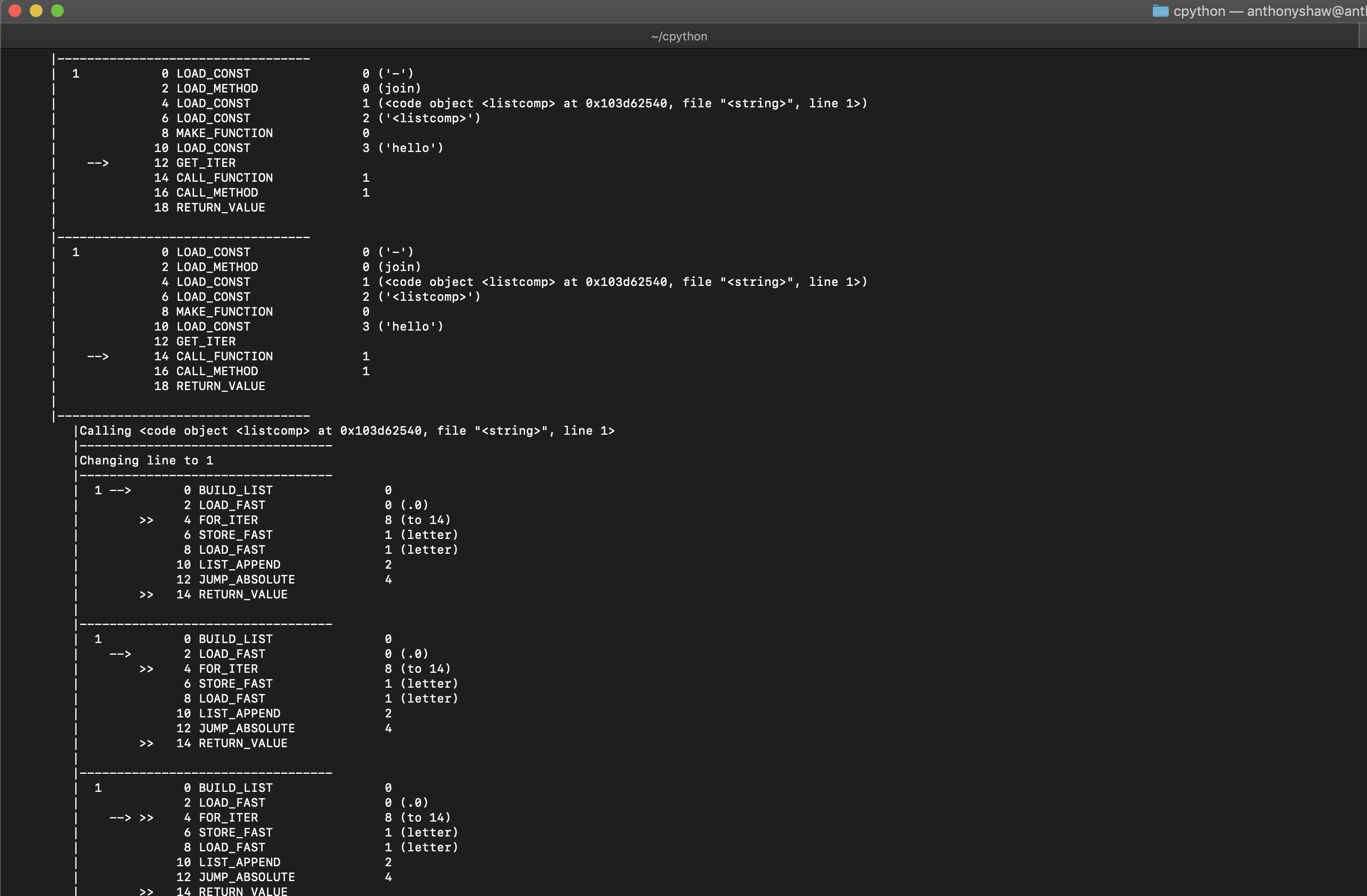
The full list of instructions is available on the dis module documentation.
Inside the core evaluation loop, a value stack is created. This stack is a list of pointers to sequential PyObject instances.
One way to think of the value stack is like a wooden peg on which you can stack cylinders. You would only add or remove one item at a time. This is done using the PUSH(a) macro, where a is a pointer to a PyObject.
For example, if you created a PyLong with the value 10 and pushed it onto the value stack:
PyObject *a = PyLong_FromLong(10);
PUSH(a);
This action would have the following effect:
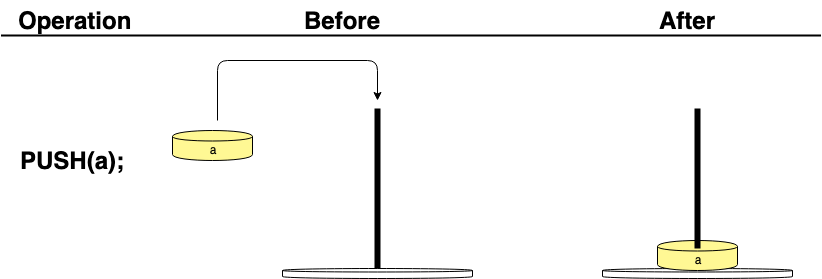
In the next operation, to fetch that value, you would use the POP() macro to take the top value from the stack:
PyObject *a = POP(); // a is PyLongObject with a value of 10
This action would return the top value and end up with an empty value stack:

If you were to add 2 values to the stack:
PyObject *a = PyLong_FromLong(10);
PyObject *b = PyLong_FromLong(20);
PUSH(a);
PUSH(b);
They would end up in the order in which they were added, so a would be pushed to the second position in the stack:

If you were to fetch the top value in the stack, you would get a pointer to b because it is at the top:

If you need to fetch the pointer to the top value in the stack without popping it, you can use the PEEK(v) operation, where v is the stack position:
PyObject *first = PEEK(0);
0 represents the top of the stack, 1 would be the second position:
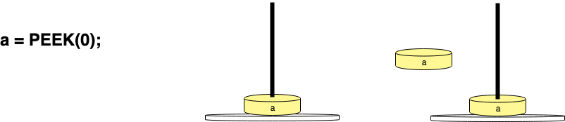
To clone the value at the top of the stack, the DUP_TWO() macro can be used, or by using the DUP_TWO opcode:
DUP_TOP();
This action would copy the value at the top to form 2 pointers to the same object:

There is a rotation macro ROT_TWO that swaps the first and second values:

Each of the opcodes have a predefined “stack effect,” calculated by the stack_effect() function inside Python/compile.c. This function returns the delta in the number of values inside the stack for each opcode.
In Python, when you create a list, the .append() method is available on the list object:
my_list = []
my_list.append(obj)
Where obj is an object, you want to append to the end of the list.
There are 2 operations involved in this operation. LOAD_FAST, to load the object obj to the top of the value stack from the list of locals in the frame, and LIST_APPEND to add the object.
First exploring LOAD_FAST, there are 5 steps:
The pointer to obj is loaded from GETLOCAL(), where the variable to load is the operation argument. The list of variable pointers is stored in fastlocals, which is a copy of the PyFrame attribute f_localsplus. The operation argument is a number, pointing to the index in the fastlocals array pointer. This means that the loading of a local is simply a copy of the pointer instead of having to look up the variable name.
If variable no longer exists, an unbound local variable error is raised.
The reference counter for value (in our case, obj) is increased by 1.
The pointer to obj is pushed to the top of the value stack.
The FAST_DISPATCH macro is called, if tracing is enabled, the loop goes over again (with all the tracing), if tracing is not enabled, a goto is called to fast_next_opcode, which jumps back to the top of the loop for the next instruction.
...
case TARGET(LOAD_FAST): {
PyObject *value = GETLOCAL(oparg); // 1.
if (value == NULL) {
format_exc_check_arg(
PyExc_UnboundLocalError,
UNBOUNDLOCAL_ERROR_MSG,
PyTuple_GetItem(co->co_varnames, oparg));
goto error; // 2.
}
Py_INCREF(value); // 3.
PUSH(value); // 4.
FAST_DISPATCH(); // 5.
}
...
Now the pointer to obj is at the top of the value stack. The next instruction LIST_APPEND is run.
Many of the bytecode operations are referencing the base types, like PyUnicode, PyNumber. For example, LIST_APPEND appends an object to the end of a list. To achieve this, it pops the pointer from the value stack and returns the pointer to the last object in the stack. The macro is a shortcut for:
PyObject *v = (*--stack_pointer);
Now the pointer to obj is stored as v. The list pointer is loaded from PEEK(oparg).
Then the C API for Python lists is called for list and v. The code for this is inside Objects/listobject.c, which we go into in the next chapter.
A call to PREDICT is made, which guesses that the next operation will be JUMP_ABSOLUTE. The PREDICT macro has compiler-generated goto statements for each of the potential operations’ case statements. This means the CPU can jump to that instruction and not have to go through the loop again:
...
case TARGET(LIST_APPEND): {
PyObject *v = POP();
PyObject *list = PEEK(oparg);
int err;
err = PyList_Append(list, v);
Py_DECREF(v);
if (err != 0)
goto error;
PREDICT(JUMP_ABSOLUTE);
DISPATCH();
}
...
Opcode predictions:
Some opcodes tend to come in pairs thus making it possible to predict the second code when the first is run. For example, COMPARE_OP is often followed by POP_JUMP_IF_FALSE or POP_JUMP_IF_TRUE.
“Verifying the prediction costs a single high-speed test of a register variable against a constant. If the pairing was good, then the processor’s own internal branch predication has a high likelihood of success, resulting in a nearly zero-overhead transition to the next opcode. A successful prediction saves a trip through the eval-loop including its unpredictable switch-case branch. Combined with the processor’s internal branch prediction, a successful PREDICT has the effect of making the two opcodes run as if they were a single new opcode with the bodies combined.”
If collecting opcode statistics, you have two choices:
Opcode prediction is disabled with threaded code since the latter allows the CPU to record separate branch prediction information for each opcode.
Some of the operations, such as CALL_FUNCTION, CALL_METHOD, have an operation argument referencing another compiled function. In these cases, another frame is pushed to the frame stack in the thread, and the evaluation loop is run for that function until the function completes. Each time a new frame is created and pushed onto the stack, the value of the frame’s f_back is set to the current frame before the new one is created.
This nesting of frames is clear when you see a stack trace, take this example script:
def function2():
raise RuntimeError
def function1():
function2()
if __name__ == '__main__':
function1()
Calling this on the command line will give you:
$ ./python.exe example_stack.py
Traceback (most recent call last):
File "example_stack.py", line 8, in <module>
function1()
File "example_stack.py", line 5, in function1
function2()
File "example_stack.py", line 2, in function2
raise RuntimeError
RuntimeError
In traceback.py, the walk_stack() function used to print trace backs:
def walk_stack(f):
"""Walk a stack yielding the frame and line number for each frame.
This will follow f.f_back from the given frame. If no frame is given, the
current stack is used. Usually used with StackSummary.extract.
"""
if f is None:
f = sys._getframe().f_back.f_back
while f is not None:
yield f, f.f_lineno
f = f.f_back
Here you can see that the current frame, fetched by calling sys._getframe() and the parent’s parent is set as the frame, because you don’t want to see the call to walk_stack() or print_trace() in the trace back, so those function frames are skipped.
Then the f_back pointer is followed to the top.
sys._getframe() is the Python API to get the frame attribute of the current thread.
Here is how that frame stack would look visually, with 3 frames each with its code object and a thread state pointing to the current frame:

In this Part, you explored the most complex element of CPython: the compiler. The original author of Python, Guido van Rossum, made the statement that CPython’s compiler should be “dumb” so that people can understand it.
By breaking down the compilation process into small, logical steps, it is far easier to understand.
In the next chapter, we connect the compilation process with the basis of all Python code, the object.
CPython comes with a collection of basic types like strings, lists, tuples, dictionaries, and objects.
All of these types are built-in. You don’t need to import any libraries, even from the standard library. Also, the instantiation of these built-in types has some handy shortcuts.
For example, to create a new list, you can call:
lst = list()
Or, you can use square brackets:
lst = []
Strings can be instantiated from a string-literal by using either double or single quotes. We explored the grammar definitions earlier that cause the compiler to interpret double quotes as a string literal.
All types in Python inherit from object, a built-in base type. Even strings, tuples, and list inherit from object. During the walk-through of the C code, you have read lots of references to PyObject*, the C-API structure for an object.
Because C is not object-oriented like Python, objects in C don’t inherit from one another. PyObject is the data structure for the beginning of the Python object’s memory.
Much of the base object API is declared in Objects/object.c, like the function PyObject_Repr, which the built-in repr() function. You will also find PyObject_Hash() and other APIs.
All of these functions can be overridden in a custom object by implementing “dunder” methods on a Python object:
class MyObject(object):
def __init__(self, id, name):
self.id = id
self.name = name
def __repr__(self):
return "<{0} id={1}>".format(self.name, self.id)
This code is implemented in PyObject_Repr(), inside Objects/object.c. The type of the target object, v will be inferred through a call to Py_TYPE() and if the tp_repr field is set, then the function pointer is called.
If the tp_repr field is not set, i.e. the object doesn’t declare a custom __repr__ method, then the default behavior is run, which is to return "<%s object at %p>" with the type name and the ID:
PyObject *
PyObject_Repr(PyObject *v)
{
PyObject *res;
if (PyErr_CheckSignals())
return NULL;
...
if (v == NULL)
return PyUnicode_FromString("<NULL>");
if (Py_TYPE(v)->tp_repr == NULL)
return PyUnicode_FromFormat("<%s object at %p>",
v->ob_type->tp_name, v);
...
}
The ob_type field for a given PyObject* will point to the data structure PyTypeObject, defined in Include/cpython/object.h.
This data-structure lists all the built-in functions, as fields and the arguments they should receive.
Take tp_repr as an example:
typedef struct _typeobject {
PyObject_VAR_HEAD
const char *tp_name; /* For printing, in format "<module>.<name>" */
Py_ssize_t tp_basicsize, tp_itemsize; /* For allocation */
/* Methods to implement standard operations */
...
reprfunc tp_repr;
Where reprfunc is a typedef for PyObject *(*reprfunc)(PyObject *);, a function that takes 1 pointer to PyObject (self).
Some of the dunder APIs are optional, because they only apply to certain types, like numbers:
/* Method suites for standard classes */
PyNumberMethods *tp_as_number;
PySequenceMethods *tp_as_sequence;
PyMappingMethods *tp_as_mapping;
A sequence, like a list would implement the following methods:
typedef struct {
lenfunc sq_length; // len(v)
binaryfunc sq_concat; // v + x
ssizeargfunc sq_repeat; // for x in v
ssizeargfunc sq_item; // v[x]
void *was_sq_slice; // v[x:y:z]
ssizeobjargproc sq_ass_item; // v[x] = z
void *was_sq_ass_slice; // v[x:y] = z
objobjproc sq_contains; // x in v
binaryfunc sq_inplace_concat;
ssizeargfunc sq_inplace_repeat;
} PySequenceMethods;
All of these built-in functions are called the Python Data Model. One of the great resources for the Python Data Model is “Fluent Python” by Luciano Ramalho.
In Objects/object.c, the base implementation of object type is written as pure C code. There are some concrete implementations of basic logic, like shallow comparisons.
Not all methods in a Python object are part of the Data Model, so that a Python object can contain attributes (either class or instance attributes) and methods.
A simple way to think of a Python object is consisting of 2 things:
The core data model is defined in the PyTypeObject, and the functions are defined in:
Objects/object.c for the built-in methodsObjects/boolobject.c for the bool typeObjects/bytearrayobject.c for the byte[] typeObjects/bytesobjects.c for the bytes typeObjects/cellobject.c for the cell typeObjects/classobject.c for the abstract class type, used in meta-programmingObjects/codeobject.c used for the built-in code object typeObjects/complexobject.c for a complex numeric typeObjects/iterobject.c for an iteratorObjects/listobject.c for the list typeObjects/longobject.c for the long numeric typeObjects/memoryobject.c for the base memory typeObjects/methodobject.c for the class method typeObjects/moduleobject.c for a module typeObjects/namespaceobject.c for a namespace typeObjects/odictobject.c for an ordered dictionary typeObjects/rangeobject.c for a range generatorObjects/setobject.c for a set typeObjects/sliceobject.c for a slice reference typeObjects/structseq.c for a struct.Struct typeObjects/tupleobject.c for a tuple typeObjects/typeobject.c for a type typeObjects/unicodeobject.c for a str typeObjects/weakrefobject.c for a weakref objectWe’re going to dive into 3 of these types:
Booleans and Integers have a lot in common, so we’ll cover those first.
The bool type is the most straightforward implementation of the built-in types. It inherits from long and has the predefined constants, Py_True and Py_False. These constants are immutable instances, created on the instantiation of the Python interpreter.
Inside Objects/boolobject.c, you can see the helper function to create a bool instance from a number:
PyObject *PyBool_FromLong(long ok)
{
PyObject *result;
if (ok)
result = Py_True;
else
result = Py_False;
Py_INCREF(result);
return result;
}
This function uses the C evaluation of a numeric type to assign Py_True or Py_False to a result and increment the reference counters.
The numeric functions for and, xor, and or are implemented, but addition, subtraction, and division are dereferenced from the base long type since it would make no sense to divide two boolean values.
The implementation of and for a bool value checks if a and b are booleans, then check their references to Py_True, otherwise, are cast as numbers, and the and operation is run on the two numbers:
static PyObject *
bool_and(PyObject *a, PyObject *b)
{
if (!PyBool_Check(a) || !PyBool_Check(b))
return PyLong_Type.tp_as_number->nb_and(a, b);
return PyBool_FromLong((a == Py_True) & (b == Py_True));
}
The long type is a bit more complex, as the memory requirements are expansive. In the transition from Python 2 to 3, CPython dropped support for the int type and instead used the long type as the primary integer type. Python’s long type is quite special in that it can store a variable-length number. The maximum length is set in the compiled binary.
The data structure of a Python long consists of the PyObject header and a list of digits. The list of digits, ob_digit is initially set to have one digit, but it later expanded to a longer length when initialized:
struct _longobject {
PyObject_VAR_HEAD
digit ob_digit[1];
};
Memory is allocated to a new long through _PyLong_New(). This function takes a fixed length and makes sure it is smaller than MAX_LONG_DIGITS. Then it reallocates the memory for ob_digit to match the length.
To convert a C long type to a Python long type, the long is converted to a list of digits, the memory for the Python long is assigned, and then each of the digits is set.
Because long is initialized with ob_digit already being at a length of 1, if the number is less than 10, then the value is set without the memory being allocated:
PyObject *
PyLong_FromLong(long ival)
{
PyLongObject *v;
unsigned long abs_ival;
unsigned long t; /* unsigned so >> doesn't propagate sign bit */
int ndigits = 0;
int sign;
CHECK_SMALL_INT(ival);
...
/* Fast path for single-digit ints */
if (!(abs_ival >> PyLong_SHIFT)) {
v = _PyLong_New(1);
if (v) {
Py_SIZE(v) = sign;
v->ob_digit[0] = Py_SAFE_DOWNCAST(
abs_ival, unsigned long, digit);
}
return (PyObject*)v;
}
...
/* Larger numbers: loop to determine number of digits */
t = abs_ival;
while (t) {
++ndigits;
t >>= PyLong_SHIFT;
}
v = _PyLong_New(ndigits);
if (v != NULL) {
digit *p = v->ob_digit;
Py_SIZE(v) = ndigits*sign;
t = abs_ival;
while (t) {
*p++ = Py_SAFE_DOWNCAST(
t & PyLong_MASK, unsigned long, digit);
t >>= PyLong_SHIFT;
}
}
return (PyObject *)v;
}
To convert a double-point floating point to a Python long, PyLong_FromDouble() does the math for you:
PyObject *
PyLong_FromDouble(double dval)
{
PyLongObject *v;
double frac;
int i, ndig, expo, neg;
neg = 0;
if (Py_IS_INFINITY(dval)) {
PyErr_SetString(PyExc_OverflowError,
"cannot convert float infinity to integer");
return NULL;
}
if (Py_IS_NAN(dval)) {
PyErr_SetString(PyExc_ValueError,
"cannot convert float NaN to integer");
return NULL;
}
if (dval < 0.0) {
neg = 1;
dval = -dval;
}
frac = frexp(dval, &expo); /* dval = frac*2**expo; 0.0 <= frac < 1.0 */
if (expo <= 0)
return PyLong_FromLong(0L);
ndig = (expo-1) / PyLong_SHIFT + 1; /* Number of 'digits' in result */
v = _PyLong_New(ndig);
if (v == NULL)
return NULL;
frac = ldexp(frac, (expo-1) % PyLong_SHIFT + 1);
for (i = ndig; --i >= 0; ) {
digit bits = (digit)frac;
v->ob_digit[i] = bits;
frac = frac - (double)bits;
frac = ldexp(frac, PyLong_SHIFT);
}
if (neg)
Py_SIZE(v) = -(Py_SIZE(v));
return (PyObject *)v;
}
The remainder of the implementation functions in longobject.c have utilities, such as converting a Unicode string into a number with PyLong_FromUnicodeObject().
Python Generators are functions which return a yield statement and can be called continually to generate further values.
Commonly they are used as a more memory efficient way of looping through values in a large block of data, like a file, a database or over a network.
Generator objects are returned in place of a value when yield is used instead of return. The generator object is created from the yield statement and returned to the caller.
Let’s create a simple generator with a list of 4 constant values:
>>> def example():
... lst = [1,2,3,4]
... for i in lst:
... yield i
...
>>> gen = example()
>>> gen
<generator object example at 0x100bcc480>
If you explore the contents of the generator object, you can see some of the fields starting with gi_:
>>> dir(gen)
[ ...
'close',
'gi_code',
'gi_frame',
'gi_running',
'gi_yieldfrom',
'send',
'throw']
The PyGenObject type is defined in Include/genobject.h and there are 3 flavors:
All 3 share the same subset of fields used in generators, and have similar behaviors:

Focusing first on generators, you can see the fields:
gi_frame linking to a PyFrameObject for the generator, earlier in the execution chapter, we explored the use of locals and globals inside a frame’s value stack. This is how generators remember the last value of local variables since the frame is persistent between callsgi_running set to 0 or 1 if the generator is currently runninggi_code linking to a PyCodeObject with the compiled function that yielded the generator so that it can be called againgi_weakreflist linking to a list of weak references to objects inside the generator functiongi_name as the name of the generatorgi_qualname as the qualified name of the generatorgi_exc_state as a tuple of exception data if the generator call raises an exceptionThe coroutine and async generators have the same fields but prepended with cr and ag respectively.
If you call __next__() on the generator object, the next value is yielded until eventually a StopIteration is raised:
>>> gen.__next__()
1
>>> gen.__next__()
2
>>> gen.__next__()
3
>>> gen.__next__()
4
>>> gen.__next__()
Traceback (most recent call last):
File "<stdin>", line 1, in <module>
StopIteration
Each time __next__() is called, the code object inside the generators gi_code field is executed as a new frame and the return value is pushed to the value stack.
You can also see that gi_code is the compiled code object for the generator function by importing the dis module and disassembling the bytecode inside:
>>> gen = example()
>>> import dis
>>> dis.disco(gen.gi_code)
2 0 LOAD_CONST 1 (1)
2 LOAD_CONST 2 (2)
4 LOAD_CONST 3 (3)
6 LOAD_CONST 4 (4)
8 BUILD_LIST 4
10 STORE_FAST 0 (l)
3 12 SETUP_LOOP 18 (to 32)
14 LOAD_FAST 0 (l)
16 GET_ITER
>> 18 FOR_ITER 10 (to 30)
20 STORE_FAST 1 (i)
4 22 LOAD_FAST 1 (i)
24 YIELD_VALUE
26 POP_TOP
28 JUMP_ABSOLUTE 18
>> 30 POP_BLOCK
>> 32 LOAD_CONST 0 (None)
34 RETURN_VALUE
Whenever __next__() is called on a generator object, gen_iternext() is called with the generator instance, which immediately calls gen_send_ex() inside Objects/genobject.c.
gen_send_ex() is the function that converts a generator object into the next yielded result. You’ll see many similarities with the way frames are constructed in Python/ceval.c from a code object as these functions have similar tasks.
The gen_send_ex() function is shared with generators, coroutines, and async generators and has the following steps:
The current thread state is fetched
The frame object from the generator object is fetched
If the generator is running when __next__() was called, raise a ValueError
If the frame inside the generator is at the top of the stack:
RuntimeError is raisedStopAsyncIterationStopIteration is raised.If the last instruction in the frame (f->f_lasti) is still -1 because it has just been started, and this is a coroutine or async generator, then a non-None value can’t be passed as an argument, so an exception is raised
Else, this is the first time it’s being called, and arguments are allowed. The value of the argument is pushed to the frame’s value stack
The f_back field of the frame is the caller to which return values are sent, so this is set to the current frame in the thread. This means that the return value is sent to the caller, not the creator of the generator
The generator is marked as running
The last exception in the generator’s exception info is copied from the last exception in the thread state
The thread state exception info is set to the address of the generator’s exception info. This means that if the caller enters a breakpoint around the execution of a generator, the stack trace goes through the generator and the offending code is clear
The frame inside the generator is executed within the Python/ceval.c main execution loop, and the value returned
The thread state last exception is reset to the value before the frame was called
The generator is marked as not running
The following cases then match the return value and any exceptions thrown by the call to the generator. Remember that generators should raise a StopIteration when they are exhausted, either manually, or by not yielding a value. Coroutines and async generators should not:
StopIteration for generators and StopAsyncIteration for async generatorsStopIteration was explicitly raised, but this is a coroutine or an async generator, raise a RuntimeError as this is not allowedStopAsyncIteration was explicitly raised and this is an async generator, raise a RuntimeError, as this is not allowedLastly, the result is returned back to the caller of __next__()
static PyObject *
gen_send_ex(PyGenObject *gen, PyObject *arg, int exc, int closing)
{
PyThreadState *tstate = _PyThreadState_GET(); // 1.
PyFrameObject *f = gen->gi_frame; // 2.
PyObject *result;
if (gen->gi_running) { // 3.
const char *msg = "generator already executing";
if (PyCoro_CheckExact(gen)) {
msg = "coroutine already executing";
}
else if (PyAsyncGen_CheckExact(gen)) {
msg = "async generator already executing";
}
PyErr_SetString(PyExc_ValueError, msg);
return NULL;
}
if (f == NULL || f->f_stacktop == NULL) { // 4.
if (PyCoro_CheckExact(gen) && !closing) {
/* `gen` is an exhausted coroutine: raise an error,
except when called from gen_close(), which should
always be a silent method. */
PyErr_SetString(
PyExc_RuntimeError,
"cannot reuse already awaited coroutine"); // 4a.
}
else if (arg && !exc) {
/* `gen` is an exhausted generator:
only set exception if called from send(). */
if (PyAsyncGen_CheckExact(gen)) {
PyErr_SetNone(PyExc_StopAsyncIteration); // 4b.
}
else {
PyErr_SetNone(PyExc_StopIteration); // 4c.
}
}
return NULL;
}
if (f->f_lasti == -1) {
if (arg && arg != Py_None) { // 5.
const char *msg = "can't send non-None value to a "
"just-started generator";
if (PyCoro_CheckExact(gen)) {
msg = NON_INIT_CORO_MSG;
}
else if (PyAsyncGen_CheckExact(gen)) {
msg = "can't send non-None value to a "
"just-started async generator";
}
PyErr_SetString(PyExc_TypeError, msg);
return NULL;
}
} else { // 6.
/* Push arg onto the frame's value stack */
result = arg ? arg : Py_None;
Py_INCREF(result);
*(f->f_stacktop++) = result;
}
/* Generators always return to their most recent caller, not
* necessarily their creator. */
Py_XINCREF(tstate->frame);
assert(f->f_back == NULL);
f->f_back = tstate->frame; // 7.
gen->gi_running = 1; // 8.
gen->gi_exc_state.previous_item = tstate->exc_info; // 9.
tstate->exc_info = &gen->gi_exc_state; // 10.
result = PyEval_EvalFrameEx(f, exc); // 11.
tstate->exc_info = gen->gi_exc_state.previous_item; // 12.
gen->gi_exc_state.previous_item = NULL;
gen->gi_running = 0; // 13.
/* Don't keep the reference to f_back any longer than necessary. It
* may keep a chain of frames alive or it could create a reference
* cycle. */
assert(f->f_back == tstate->frame);
Py_CLEAR(f->f_back);
/* If the generator just returned (as opposed to yielding), signal
* that the generator is exhausted. */
if (result && f->f_stacktop == NULL) { // 14a.
if (result == Py_None) {
/* Delay exception instantiation if we can */
if (PyAsyncGen_CheckExact(gen)) {
PyErr_SetNone(PyExc_StopAsyncIteration);
}
else {
PyErr_SetNone(PyExc_StopIteration);
}
}
else {
/* Async generators cannot return anything but None */
assert(!PyAsyncGen_CheckExact(gen));
_PyGen_SetStopIterationValue(result);
}
Py_CLEAR(result);
}
else if (!result && PyErr_ExceptionMatches(PyExc_StopIteration)) { // 14b.
const char *msg = "generator raised StopIteration";
if (PyCoro_CheckExact(gen)) {
msg = "coroutine raised StopIteration";
}
else if PyAsyncGen_CheckExact(gen) {
msg = "async generator raised StopIteration";
}
_PyErr_FormatFromCause(PyExc_RuntimeError, "%s", msg);
}
else if (!result && PyAsyncGen_CheckExact(gen) &&
PyErr_ExceptionMatches(PyExc_StopAsyncIteration)) // 14c.
{
/* code in `gen` raised a StopAsyncIteration error:
raise a RuntimeError.
*/
const char *msg = "async generator raised StopAsyncIteration";
_PyErr_FormatFromCause(PyExc_RuntimeError, "%s", msg);
}
...
return result; // 15.
}
Going back to the evaluation of code objects whenever a function or module is called, there was a special case for generators, coroutines, and async generators in _PyEval_EvalCodeWithName(). This function checks for the CO_GENERATOR, CO_COROUTINE, and CO_ASYNC_GENERATOR flags on the code object.
When a new coroutine is created using PyCoro_New(), a new async generator is created with PyAsyncGen_New() or a generator with PyGen_NewWithQualName(). These objects are returned early instead of returning an evaluated frame, which is why you get a generator object after calling a function with a yield statement:
PyObject *
_PyEval_EvalCodeWithName(PyObject *_co, PyObject *globals, PyObject *locals, ...
...
/* Handle generator/coroutine/asynchronous generator */
if (co->co_flags & (CO_GENERATOR | CO_COROUTINE | CO_ASYNC_GENERATOR)) {
PyObject *gen;
PyObject *coro_wrapper = tstate->coroutine_wrapper;
int is_coro = co->co_flags & CO_COROUTINE;
...
/* Create a new generator that owns the ready to run frame
* and return that as the value. */
if (is_coro) {
gen = PyCoro_New(f, name, qualname);
} else if (co->co_flags & CO_ASYNC_GENERATOR) {
gen = PyAsyncGen_New(f, name, qualname);
} else {
gen = PyGen_NewWithQualName(f, name, qualname);
}
...
return gen;
}
...
The flags in the code object were injected by the compiler after traversing the AST and seeing the yield or yield from statements or seeing the coroutine decorator.
PyGen_NewWithQualName() will call gen_new_with_qualname() with the generated frame and then create the PyGenObject with NULL values and the compiled code object:
static PyObject *
gen_new_with_qualname(PyTypeObject *type, PyFrameObject *f,
PyObject *name, PyObject *qualname)
{
PyGenObject *gen = PyObject_GC_New(PyGenObject, type);
if (gen == NULL) {
Py_DECREF(f);
return NULL;
}
gen->gi_frame = f;
f->f_gen = (PyObject *) gen;
Py_INCREF(f->f_code);
gen->gi_code = (PyObject *)(f->f_code);
gen->gi_running = 0;
gen->gi_weakreflist = NULL;
gen->gi_exc_state.exc_type = NULL;
gen->gi_exc_state.exc_value = NULL;
gen->gi_exc_state.exc_traceback = NULL;
gen->gi_exc_state.previous_item = NULL;
if (name != NULL)
gen->gi_name = name;
else
gen->gi_name = ((PyCodeObject *)gen->gi_code)->co_name;
Py_INCREF(gen->gi_name);
if (qualname != NULL)
gen->gi_qualname = qualname;
else
gen->gi_qualname = gen->gi_name;
Py_INCREF(gen->gi_qualname);
_PyObject_GC_TRACK(gen);
return (PyObject *)gen;
}
Bringing this all together you can see how the generator expression is a powerful syntax where a single keyword, yield triggers a whole flow to create a unique object, copy a compiled code object as a property, set a frame, and store a list of variables in the local scope.
To the user of the generator expression, this all seems like magic, but under the covers it’s not that complex.
Now that you understand how some built-in types, you can explore other types.
When exploring Python classes, it is important to remember there are built-in types, written in C and classes inheriting from those types, written in Python or C.
Some libraries have types written in C instead of inheriting from the built-in types. One example is numpy, a library for numeric arrays. The nparray type is written in C, is highly efficient and performant.
In the next Part, we will explore the classes and functions defined in the standard library.
Python has always come “batteries included.” This statement means that with a standard CPython distribution, there are libraries for working with files, threads, networks, web sites, music, keyboards, screens, text, and a whole manner of utilities.
Some of the batteries that come with CPython are more like AA batteries. They’re useful for everything, like the collections module and the sys module. Some of them are a bit more obscure, like a small watch battery that you never know when it might come in useful.
There are 2 types of modules in the CPython standard library:
We will explore both types.
The modules written in pure Python are all located in the Lib/ directory in the source code. Some of the larger modules have submodules in subfolders, like the email module.
An easy module to look at would be the colorsys module. It’s only a few hundred lines of Python code. You may not have come across it before. The colorsys module has some utility functions for converting color scales.
When you install a Python distribution from source, standard library modules are copied from the Lib folder into the distribution folder. This folder is always part of your path when you start Python, so you can import the modules without having to worry about where they’re located.
For example:
>>> import colorsys
>>> colorsys
<module 'colorsys' from '/usr/shared/lib/python3.7/colorsys.py'>
>>> colorsys.rgb_to_hls(255,0,0)
(0.0, 127.5, -1.007905138339921)
We can see the source code of rgb_to_hls() inside Lib/colorsys.py:
# HLS: Hue, Luminance, Saturation
# H: position in the spectrum
# L: color lightness
# S: color saturation
def rgb_to_hls(r, g, b):
maxc = max(r, g, b)
minc = min(r, g, b)
# XXX Can optimize (maxc+minc) and (maxc-minc)
l = (minc+maxc)/2.0
if minc == maxc:
return 0.0, l, 0.0
if l <= 0.5:
s = (maxc-minc) / (maxc+minc)
else:
s = (maxc-minc) / (2.0-maxc-minc)
rc = (maxc-r) / (maxc-minc)
gc = (maxc-g) / (maxc-minc)
bc = (maxc-b) / (maxc-minc)
if r == maxc:
h = bc-gc
elif g == maxc:
h = 2.0+rc-bc
else:
h = 4.0+gc-rc
h = (h/6.0) % 1.0
return h, l, s
There’s nothing special about this function, it’s just standard Python. You’ll find similar things with all of the pure Python standard library modules. They’re just written in plain Python, well laid out and easy to understand. You may even spot improvements or bugs, so you can make changes to them and contribute it to the Python distribution. We’ll cover that toward the end of this article.
The remainder of modules are written in C, or a combination or Python and C. The source code for these is in Lib/ for the Python component, and Modules/ for the C component. There are two exceptions to this rule, the sys module, found in Python/sysmodule.c and the __builtins__ module, found in Python/bltinmodule.c.
Python will import * from __builtins__ when an interpreter is instantiated, so all of the functions like print(), chr(), format(), etc. are found within Python/bltinmodule.c.
Because the sys module is so specific to the interpreter and the internals of CPython, that is found inside the Python directly. It is also marked as an “implementation detail” of CPython and not found in other distributions.
The built-in print() function was probably the first thing you learned to do in Python. So what happens when you type print("hello world!")?
"hello world" was converted from a string constant to a PyUnicodeObject by the compilerbuiltin_print() was executed with 1 argument, and NULL kwnamesfile variable is set to PyId_stdout, the system’s stdout handlefile\n is sent to filestatic PyObject *
builtin_print(PyObject *self, PyObject *const *args, Py_ssize_t nargs, PyObject *kwnames)
{
...
if (file == NULL || file == Py_None) {
file = _PySys_GetObjectId(&PyId_stdout);
...
}
...
for (i = 0; i < nargs; i++) {
if (i > 0) {
if (sep == NULL)
err = PyFile_WriteString(" ", file);
else
err = PyFile_WriteObject(sep, file,
Py_PRINT_RAW);
if (err)
return NULL;
}
err = PyFile_WriteObject(args[i], file, Py_PRINT_RAW);
if (err)
return NULL;
}
if (end == NULL)
err = PyFile_WriteString("\n", file);
else
err = PyFile_WriteObject(end, file, Py_PRINT_RAW);
...
Py_RETURN_NONE;
}
The contents of some modules written in C expose operating system functions. Because the CPython source code needs to compile to macOS, Windows, Linux, and other *nix-based operating systems, there are some special cases.
The time module is a good example. The way that Windows keeps and stores time in the Operating System is fundamentally different than Linux and macOS. This is one of the reasons why the accuracy of the clock functions differs between operating systems.
In Modules/timemodule.c, the operating system time functions for Unix-based systems are imported from <sys/times.h>:
#ifdef HAVE_SYS_TIMES_H
#include <sys/times.h>
#endif
...
#ifdef MS_WINDOWS
#define WIN32_LEAN_AND_MEAN
#include <windows.h>
#include "pythread.h"
#endif /* MS_WINDOWS */
...
Later in the file, time_process_time_ns() is defined as a wrapper for _PyTime_GetProcessTimeWithInfo():
static PyObject *
time_process_time_ns(PyObject *self, PyObject *unused)
{
_PyTime_t t;
if (_PyTime_GetProcessTimeWithInfo(&t, NULL) < 0) {
return NULL;
}
return _PyTime_AsNanosecondsObject(t);
}
_PyTime_GetProcessTimeWithInfo() is implemented multiple different ways in the source code, but only certain parts are compiled into the binary for the module, depending on the operating system. Windows systems will call GetProcessTimes() and Unix systems will call clock_gettime().
Other modules that have multiple implementations for the same API are the threading module, the file system module, and the networking modules. Because the Operating Systems behave differently, the CPython source code implements the same behavior as best as it can and exposes it using a consistent, abstracted API.
CPython has a robust and extensive test suite covering the core interpreter, the standard library, the tooling and distribution for both Windows and Linux/macOS.
The test suite is located in Lib/test and written almost entirely in Python.
The full test suite is a Python package, so can be run using the Python interpreter that you’ve compiled. Change directory to the Lib directory and run python -m test -j2, where j2 means to use 2 CPUs.
On Windows use the rt.bat script inside the PCBuild folder, ensuring that you have built the Release configuration from Visual Studio in advance:
$ cd PCbuild
$ rt.bat -q
C:\repos\cpython\PCbuild>"C:\repos\cpython\PCbuild\win32\python.exe" -u -Wd -E -bb -m test
== CPython 3.8.0b4
== Windows-10-10.0.17134-SP0 little-endian
== cwd: C:\repos\cpython\build\test_python_2784
== CPU count: 2
== encodings: locale=cp1252, FS=utf-8
Run tests sequentially
0:00:00 [ 1/420] test_grammar
0:00:00 [ 2/420] test_opcodes
0:00:00 [ 3/420] test_dict
0:00:00 [ 4/420] test_builtin
...
On Linux:
$ cd Lib
$ ../python -m test -j2
== CPython 3.8.0b4
== macOS-10.14.3-x86_64-i386-64bit little-endian
== cwd: /Users/anthonyshaw/cpython/build/test_python_23399
== CPU count: 4
== encodings: locale=UTF-8, FS=utf-8
Run tests in parallel using 2 child processes
0:00:00 load avg: 2.14 [ 1/420] test_opcodes passed
0:00:00 load avg: 2.14 [ 2/420] test_grammar passed
...
On macOS:
$ cd Lib
$ ../python.exe -m test -j2
== CPython 3.8.0b4
== macOS-10.14.3-x86_64-i386-64bit little-endian
== cwd: /Users/anthonyshaw/cpython/build/test_python_23399
== CPU count: 4
== encodings: locale=UTF-8, FS=utf-8
Run tests in parallel using 2 child processes
0:00:00 load avg: 2.14 [ 1/420] test_opcodes passed
0:00:00 load avg: 2.14 [ 2/420] test_grammar passed
...
Some tests require certain flags; otherwise they are skipped. For example, many of the IDLE tests require a GUI.
To see a list of test suites in the configuration, use the --list-tests flag:
$ ../python.exe -m test --list-tests
test_grammar
test_opcodes
test_dict
test_builtin
test_exceptions
...
You can run specific tests by providing the test suite as the first argument:
$ ../python.exe -m test test_webbrowser
Run tests sequentially
0:00:00 load avg: 2.74 [1/1] test_webbrowser
== Tests result: SUCCESS ==
1 test OK.
Total duration: 117 ms
Tests result: SUCCESS
You can also see a detailed list of tests that were executed with the result using the -v argument:
$ ../python.exe -m test test_webbrowser -v
== CPython 3.8.0b4
== macOS-10.14.3-x86_64-i386-64bit little-endian
== cwd: /Users/anthonyshaw/cpython/build/test_python_24562
== CPU count: 4
== encodings: locale=UTF-8, FS=utf-8
Run tests sequentially
0:00:00 load avg: 2.36 [1/1] test_webbrowser
test_open (test.test_webbrowser.BackgroundBrowserCommandTest) ... ok
test_register (test.test_webbrowser.BrowserRegistrationTest) ... ok
test_register_default (test.test_webbrowser.BrowserRegistrationTest) ... ok
test_register_preferred (test.test_webbrowser.BrowserRegistrationTest) ... ok
test_open (test.test_webbrowser.ChromeCommandTest) ... ok
test_open_new (test.test_webbrowser.ChromeCommandTest) ... ok
...
test_open_with_autoraise_false (test.test_webbrowser.OperaCommandTest) ... ok
----------------------------------------------------------------------
Ran 34 tests in 0.056s
OK (skipped=2)
== Tests result: SUCCESS ==
1 test OK.
Total duration: 134 ms
Tests result: SUCCESS
Understanding how to use the test suite and checking the state of the version you have compiled is very important if you wish to make changes to CPython. Before you start making changes, you should run the whole test suite and make sure everything is passing.
From your source repository, if you’re happy with your changes and want to use them inside your system, you can install it as a custom version.
For macOS and Linux, you can use the altinstall command, which won’t create symlinks for python3 and install a standalone version:
$ make altinstall
For Windows, you have to change the build configuration from Debug to Release, then copy the packaged binaries to a directory on your computer which is part of the system path.
Congratulations, you made it! Did your tea get cold? Make yourself another cup. You’ve earned it.
Now that you’ve seen the CPython source code, the modules, the compiler, and the tooling, you may wish to make some changes and contribute them back to the Python ecosystem.
The official dev guide contains plenty of resources for beginners. You’ve already taken the first step, to understand the source, knowing how to change, compile, and test the CPython applications.
Think back to all the things you’ve learned about CPython over this article. All the pieces of magic to which you’ve learned the secrets. The journey doesn’t stop here.
This might be a good time to learn more about Python and C. Who knows: you could be contributing more and more to the CPython project!
[ Improve Your Python With 🐍 Python Tricks 💌 – Get a short & sweet Python Trick delivered to your inbox every couple of days. >> Click here to learn more and see examples ]
# datePublished: #Wed Aug 21 16:10:00 2019# dateUpdated: #Wed Aug 21 16:10:00 2019# # Person begin #################### name: #Real Python# # Person end ###################### # Item end ######################## # Item begin ###################### id: #https://realpython.com/courses/python-histograms/# title: #Python Histogram Plotting: NumPy, Matplotlib, Pandas & Seaborn# link: #https://realpython.com/courses/python-histograms/# description: #In this course, you'll be equipped to make production-quality, presentation-ready Python histogram plots with a range of choices and features. It's your one-stop shop for constructing and manipulating histograms with Python's scientific stack.# content: #In this course, you’ll be equipped to make production-quality, presentation-ready Python histogram plots with a range of choices and features.
If you have introductory to intermediate knowledge in Python and statistics, then you can use this article as a one-stop shop for building and plotting histograms in Python using libraries from its scientific stack, including NumPy, Matplotlib, Pandas, and Seaborn.
A histogram is a great tool for quickly assessing a probability distribution that is intuitively understood by almost any audience. Python offers a handful of different options for building and plotting histograms. Most people know a histogram by its graphical representation, which is similar to a bar graph:
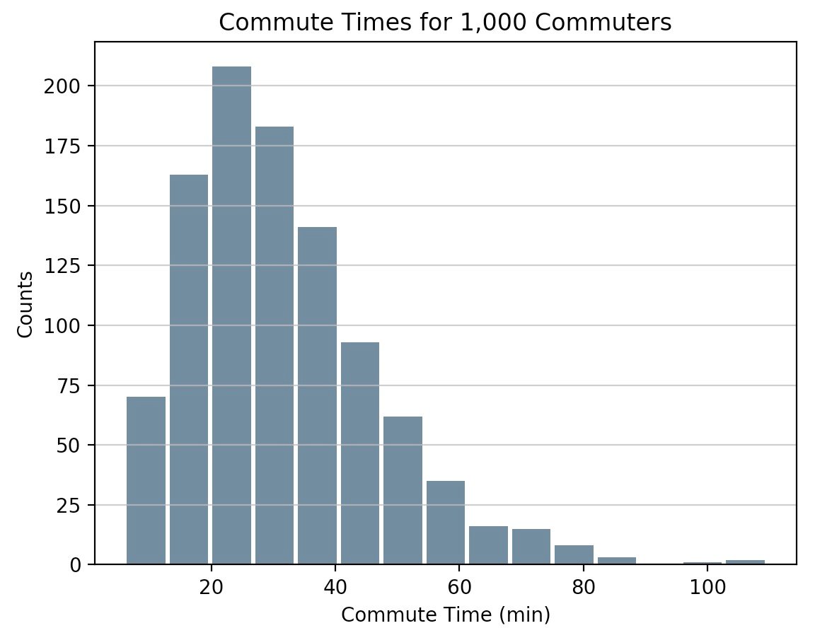
This course will guide you through creating plots like the one above as well as more complex ones. Here’s what you’ll cover:
Free Bonus: Short on time? Click here to get access to a free two-page Python histograms cheat sheet that summarizes the techniques explained in this tutorial.
[ Improve Your Python With 🐍 Python Tricks 💌 – Get a short & sweet Python Trick delivered to your inbox every couple of days. >> Click here to learn more and see examples ]
# datePublished: #Tue Aug 20 14:00:00 2019# dateUpdated: #Tue Aug 20 14:00:00 2019# # Person begin #################### name: #Real Python# # Person end ###################### # Item end ######################## # Item begin ###################### id: #https://realpython.com/how-to-make-a-discord-bot-python/# title: #How to Make a Discord Bot in Python# link: #https://realpython.com/how-to-make-a-discord-bot-python/# description: #In this step-by-step tutorial, you'll learn how to make a Discord bot in Python and interact with several APIs. You'll learn how to handle events, accept commands, validate and verify input, and all the basics that can help you create useful and exciting automations!# content: #In a world where video games are so important to so many people, communication and community around games are vital. Discord offers both of those and more in one well-designed package. In this tutorial, you’ll learn how to make a Discord bot in Python so that you can make the most of this fantastic platform.
By the end of this article you’ll learn:
You’ll begin by learning what Discord is and why it’s valuable.
Free Bonus: Click here to get access to a chapter from Python Tricks: The Book that shows you Python's best practices with simple examples you can apply instantly to write more beautiful + Pythonic code.
Discord is a voice and text communication platform for gamers.
Players, streamers, and developers use Discord to discuss games, answer questions, chat while they play, and much more. It even has a game store, complete with critical reviews and a subscription service. It is nearly a one-stop shop for gaming communities.
While there are many things you can build using Discord’s APIs, this tutorial will focus on a particular learning outcome: how to make a Discord bot in Python.
Discord is growing in popularity. As such, automated processes, such as banning inappropriate users and reacting to user requests are vital for a community to thrive and grow.
Automated programs that look and act like users and automatically respond to events and commands on Discord are called bot users. Discord bot users (or just bots) have nearly unlimited applications.
For example, let’s say you’re managing a new Discord guild and a user joins for the very first time. Excited, you may personally reach out to that user and welcome them to your community. You might also tell them about your channels or ask them to introduce themselves.
The user feels welcomed and enjoys the discussions that happen in your guild and they, in turn, invite friends.
Over time, your community grows so big that it’s no longer feasible to personally reach out to each new member, but you still want to send them something to recognize them as a new member of the guild.
With a bot, it’s possible to automatically react to the new member joining your guild. You can even customize its behavior based on context and control how it interacts with each new user.
This is great, but it’s only one small example of how a bot can be useful. There are so many opportunities for you to be creative with bots, once you know how to make them.
Note: Although Discord allows you to create bots that deal with voice communication, this article will stick to the text side of the service.
There are two key steps when you’re creating a bot:
In the next section, you’ll learn how to make a Discord bot in Discord’s Developer Portal.
Before you can dive into any Python code to handle events and create exciting automations, you need to first create a few Discord components:
You’ll learn more about each piece in the following sections.
Once you’ve created all of these components, you’ll tie them together by registering your bot with your guild.
You can get started by heading to Discord’s Developer Portal.
The first thing you’ll see is a landing page where you’ll need to either login, if you have an existing account, or create a new account:

If you need to create a new account, then click on the Register button below Login and enter your account information.
Important: You’ll need to verify your email before you’re able to move on.
Once you’re finished, you’ll be redirected to the Developer Portal home page, where you’ll create your application.
An application allows you to interact with Discord’s APIs by providing authentication tokens, designating permissions, and so on.
To create a new application, select New Application:
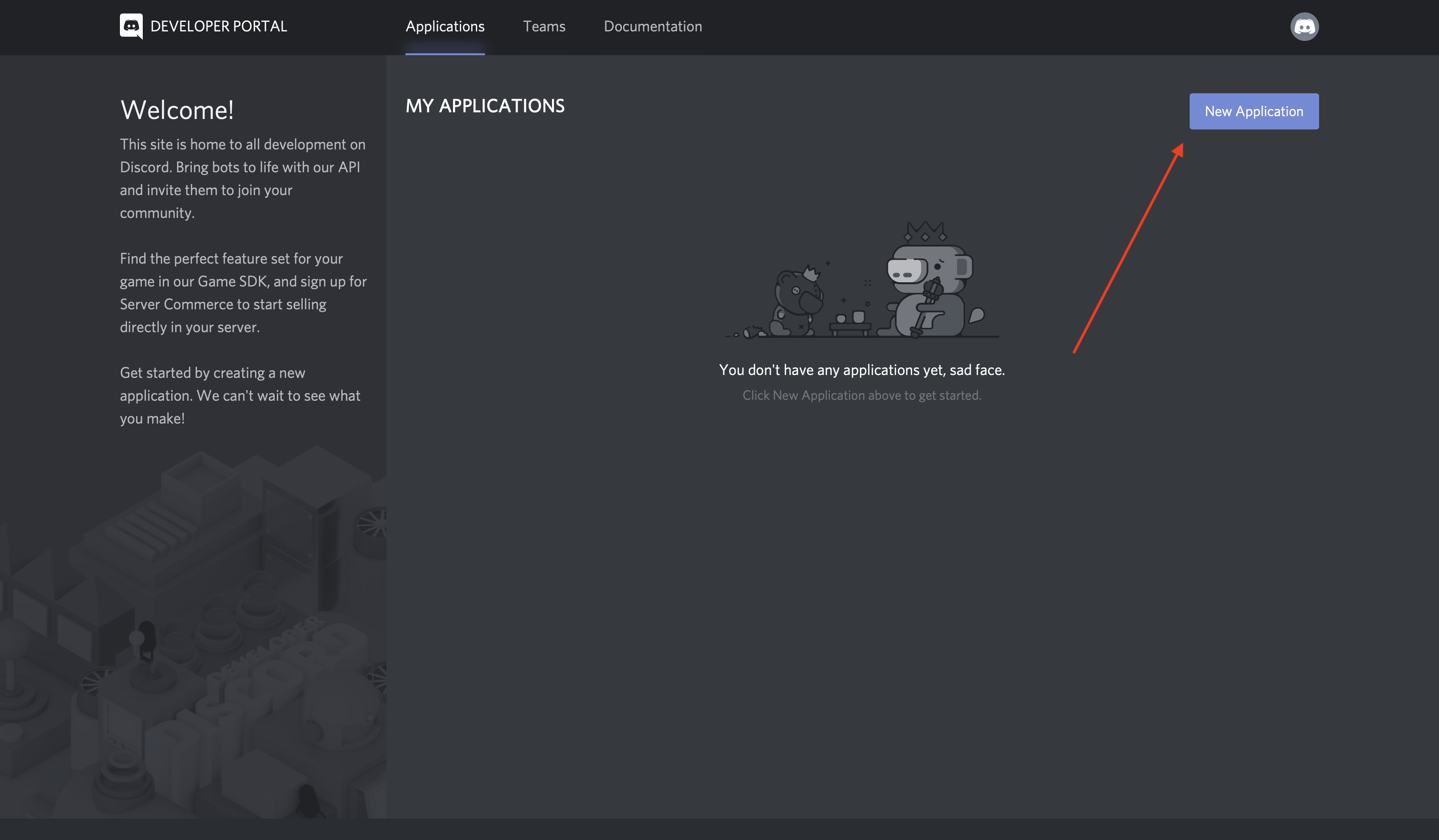
Next, you’ll be prompted to name your application. Select a name and click Create:
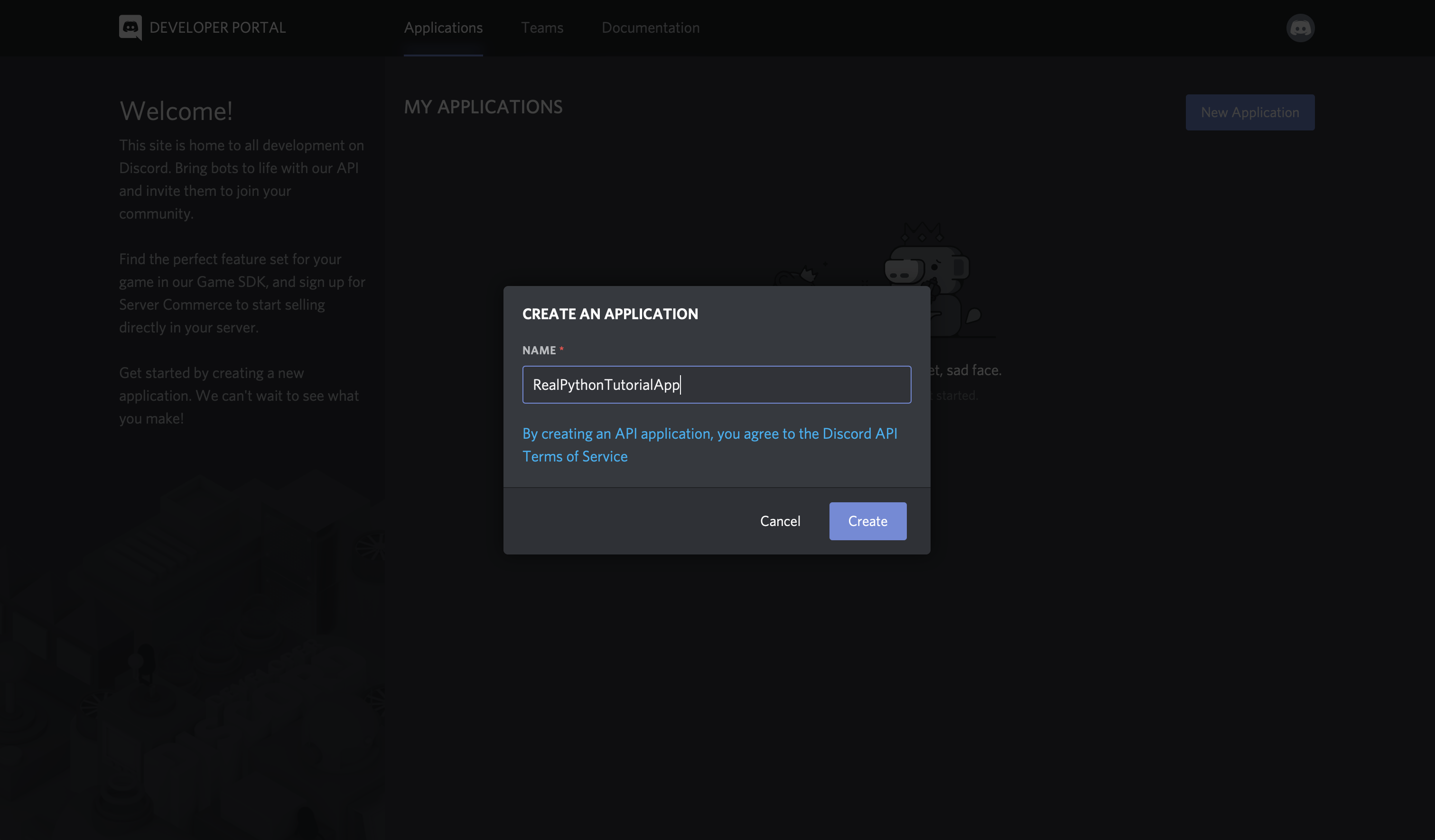
Congratulations! You made a Discord application. On the resulting screen, you can see information about your application:
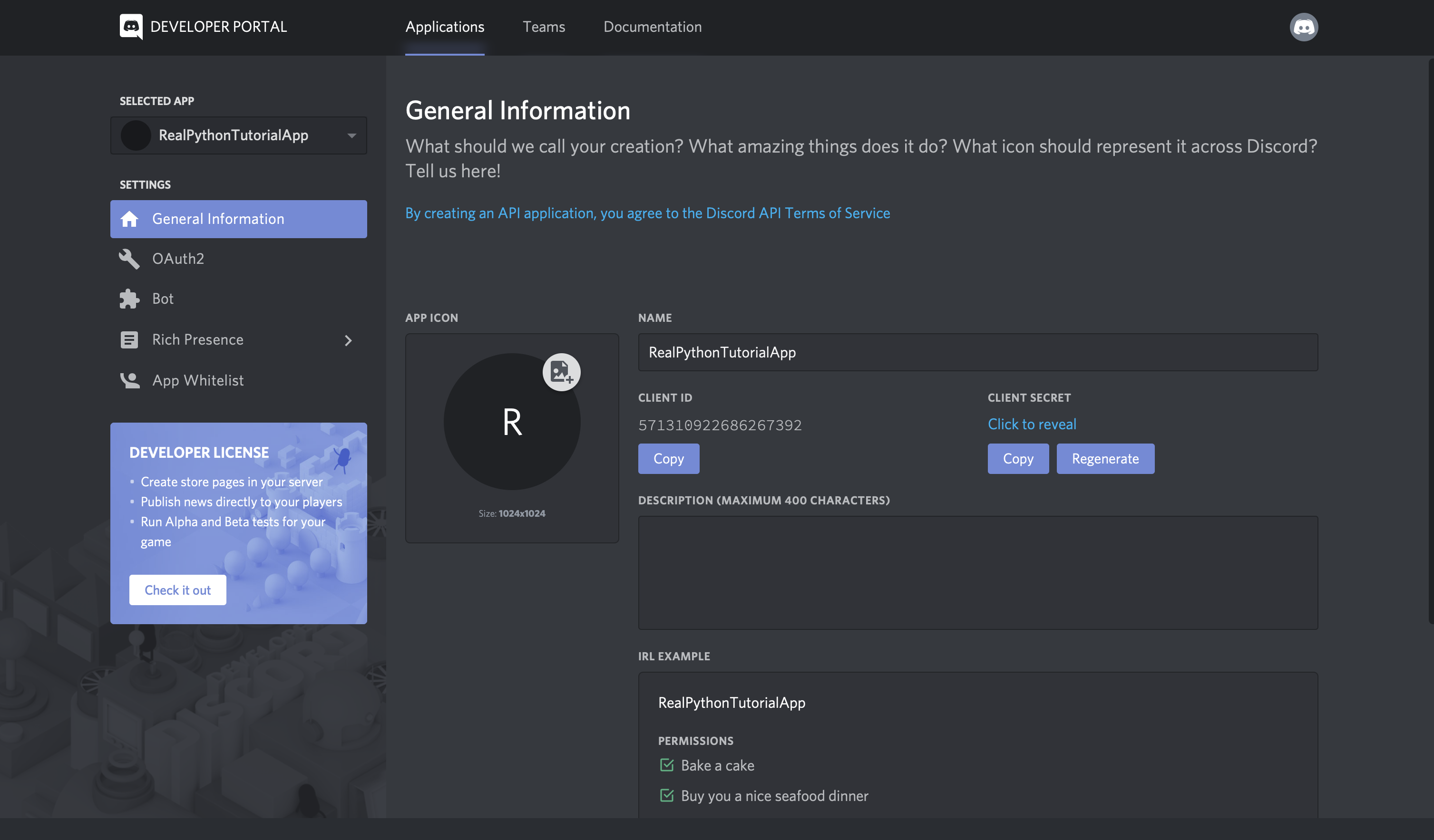
Keep in mind that any program that interacts with Discord APIs requires a Discord application, not just bots. Bot-related APIs are only a subset of Discord’s total interface.
However, since this tutorial is about how to make a Discord bot, navigate to the Bot tab on the left-hand navigation list.
As you learned in the previous sections, a bot user is one that listens to and automatically reacts to certain events and commands on Discord.
For your code to actually be manifested on Discord, you’ll need to create a bot user. To do so, select Add Bot:
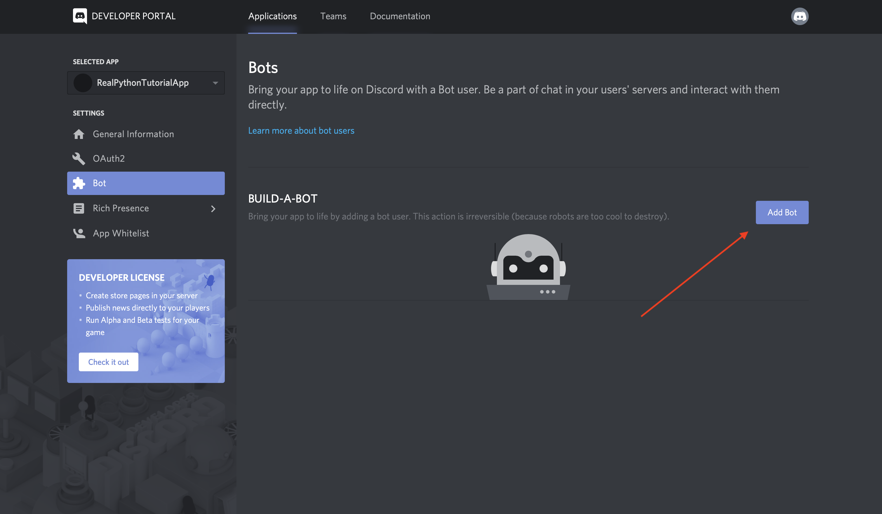
Once you confirm that you want to add the bot to your application, you’ll see the new bot user in the portal:
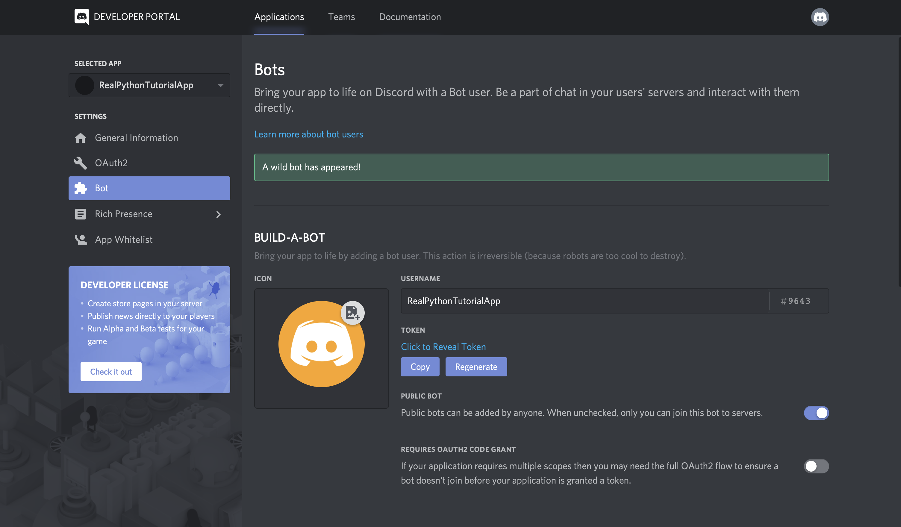
Notice that, by default, your bot user will inherit the name of your application. Instead, update the username to something more bot-like, such as RealPythonTutorialBot, and Save Changes:
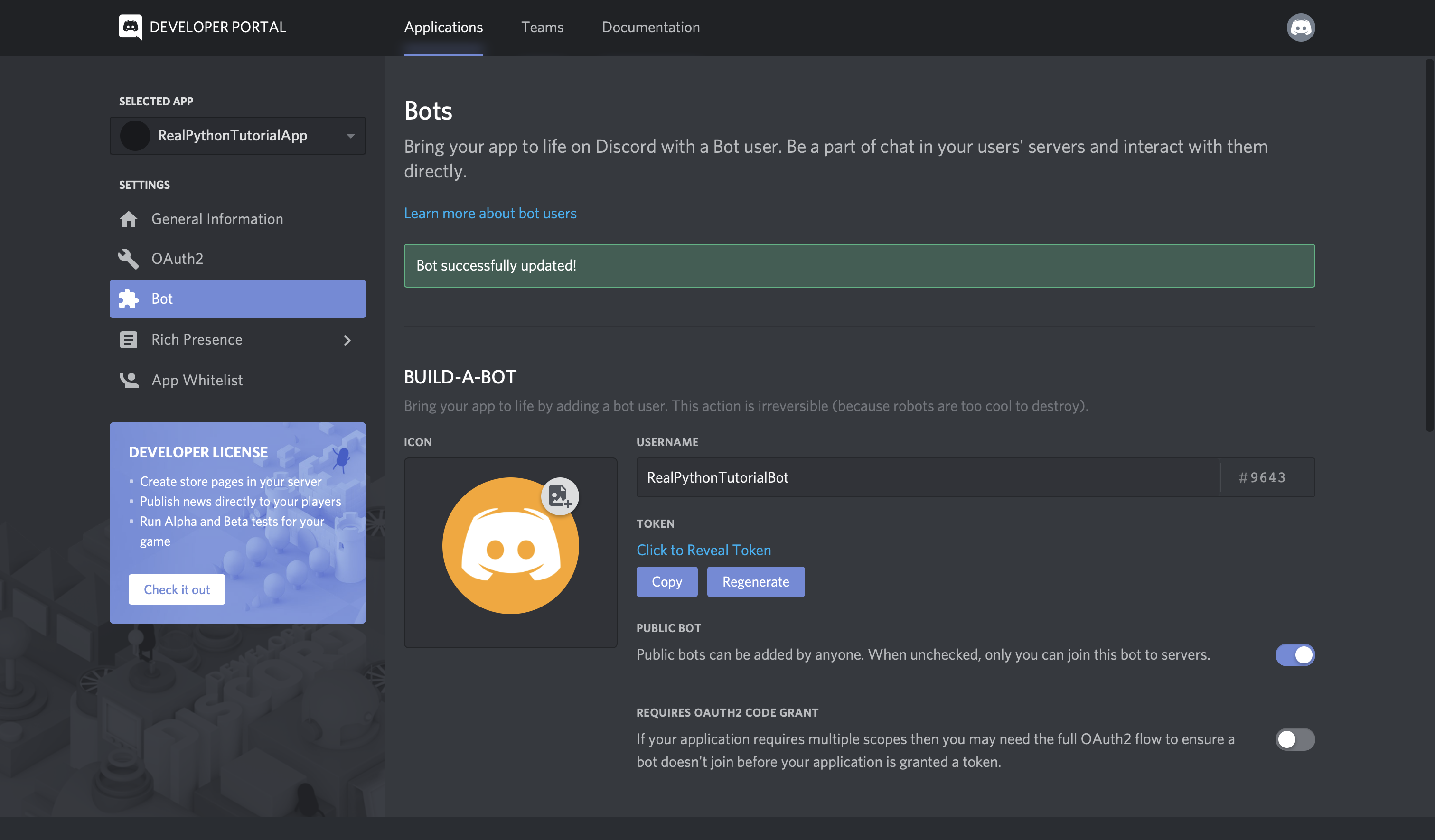
Now, the bot’s all set and ready to go, but to where?
A bot user is not useful if it’s not interacting with other users. Next, you’ll create a guild so that your bot can interact with other users.
A guild (or a server, as it is often called in Discord’s user interface) is a specific group of channels where users congregate to chat.
Note: While guild and server are interchangeable, this article will use the term guild primarily because the APIs stick to the same term. The term server will only be used when referring to a guild in the graphical UI.
For example, say you want to create a space where users can come together and talk about your latest game. You’d start by creating a guild. Then, in your guild, you could have multiple channels, such as:
Once you’ve created your guild, you’d invite other users to populate it.
So, to create a guild, head to your Discord home page:
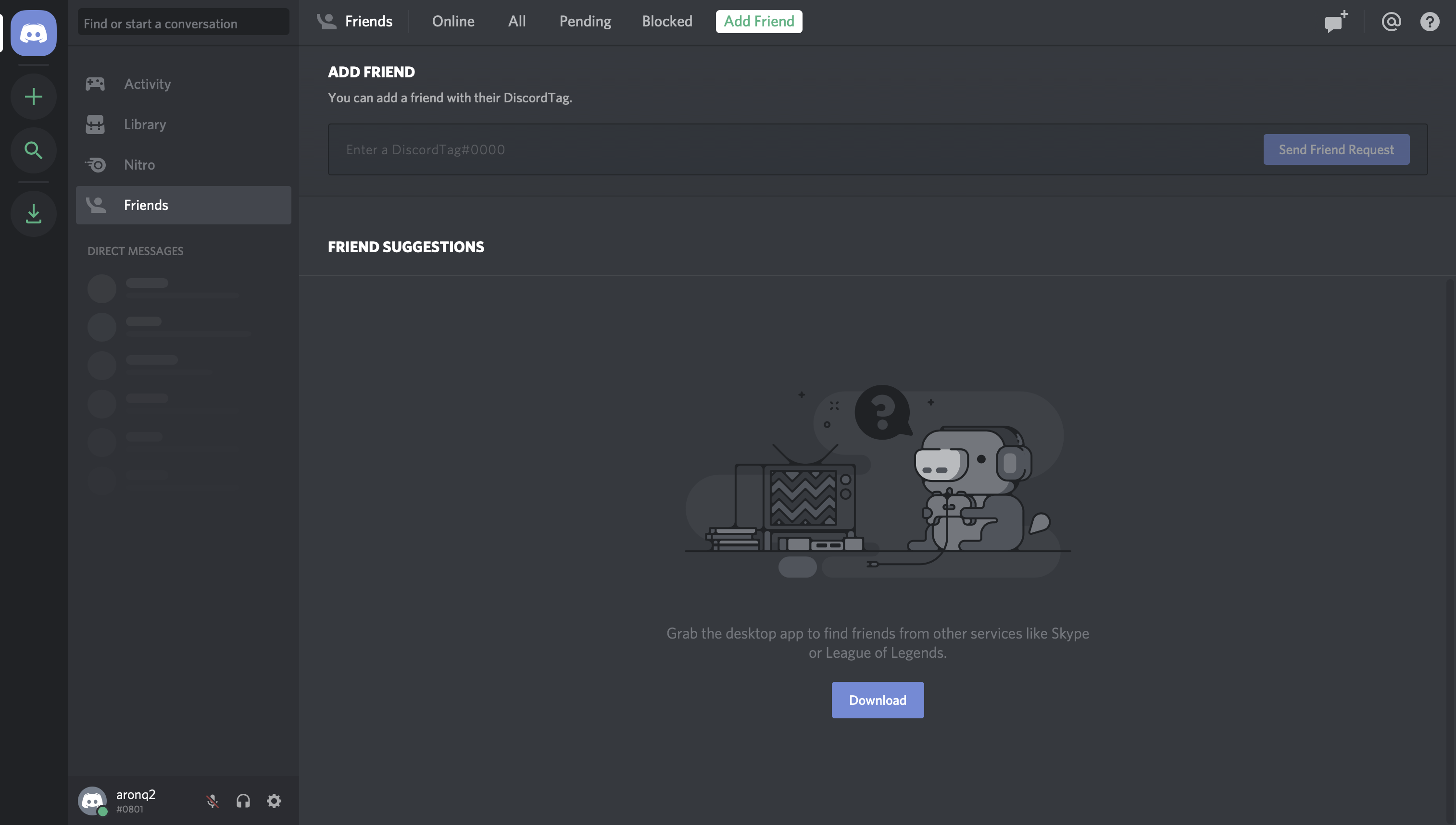
From this home page, you can view and add friends, direct messages, and guilds. From here, select the + icon on the left-hand side of the web page to Add a Server:
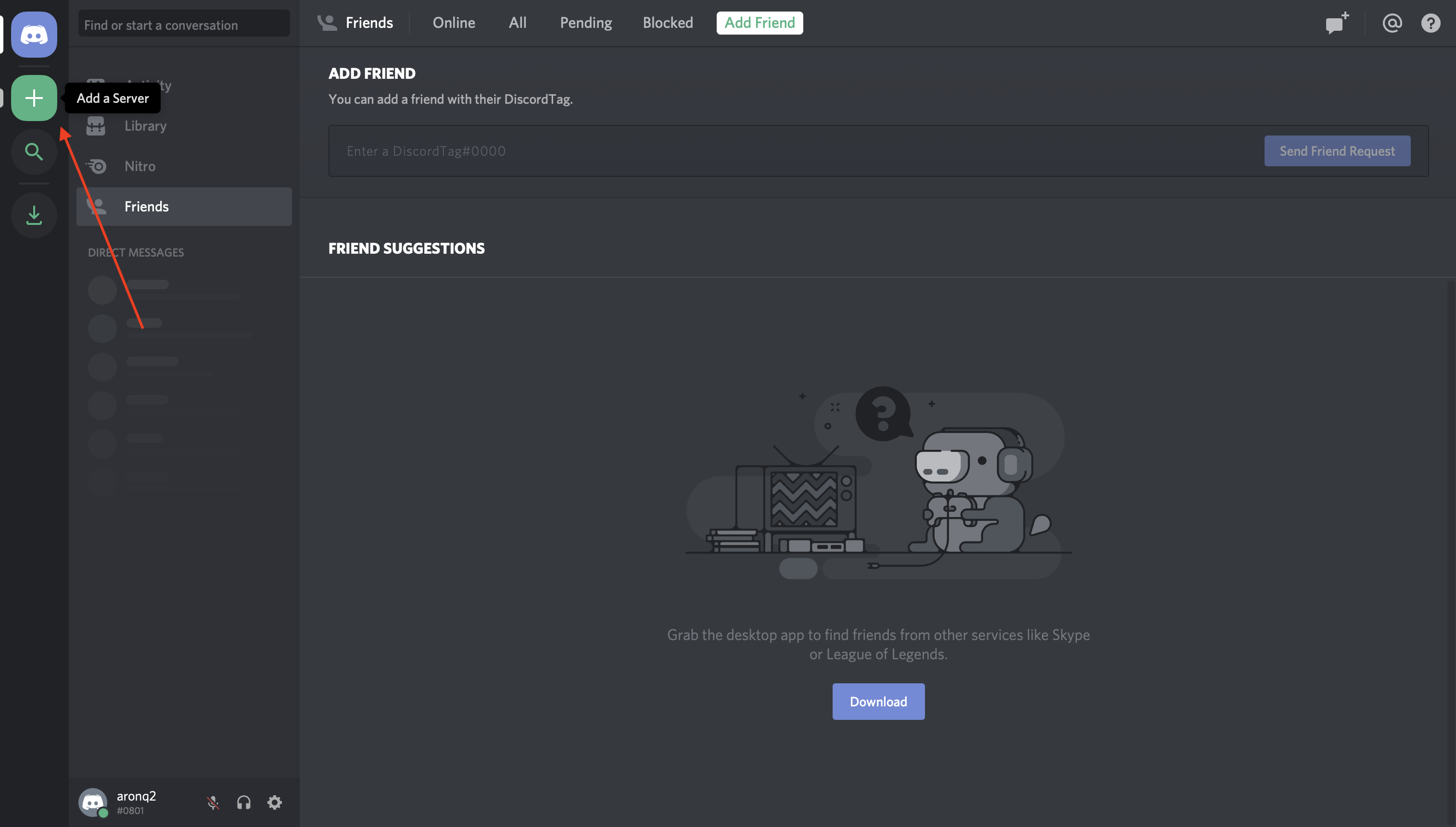
This will present two options, Create a server and Join a Server. In this case, select Create a server and enter a name for your guild:
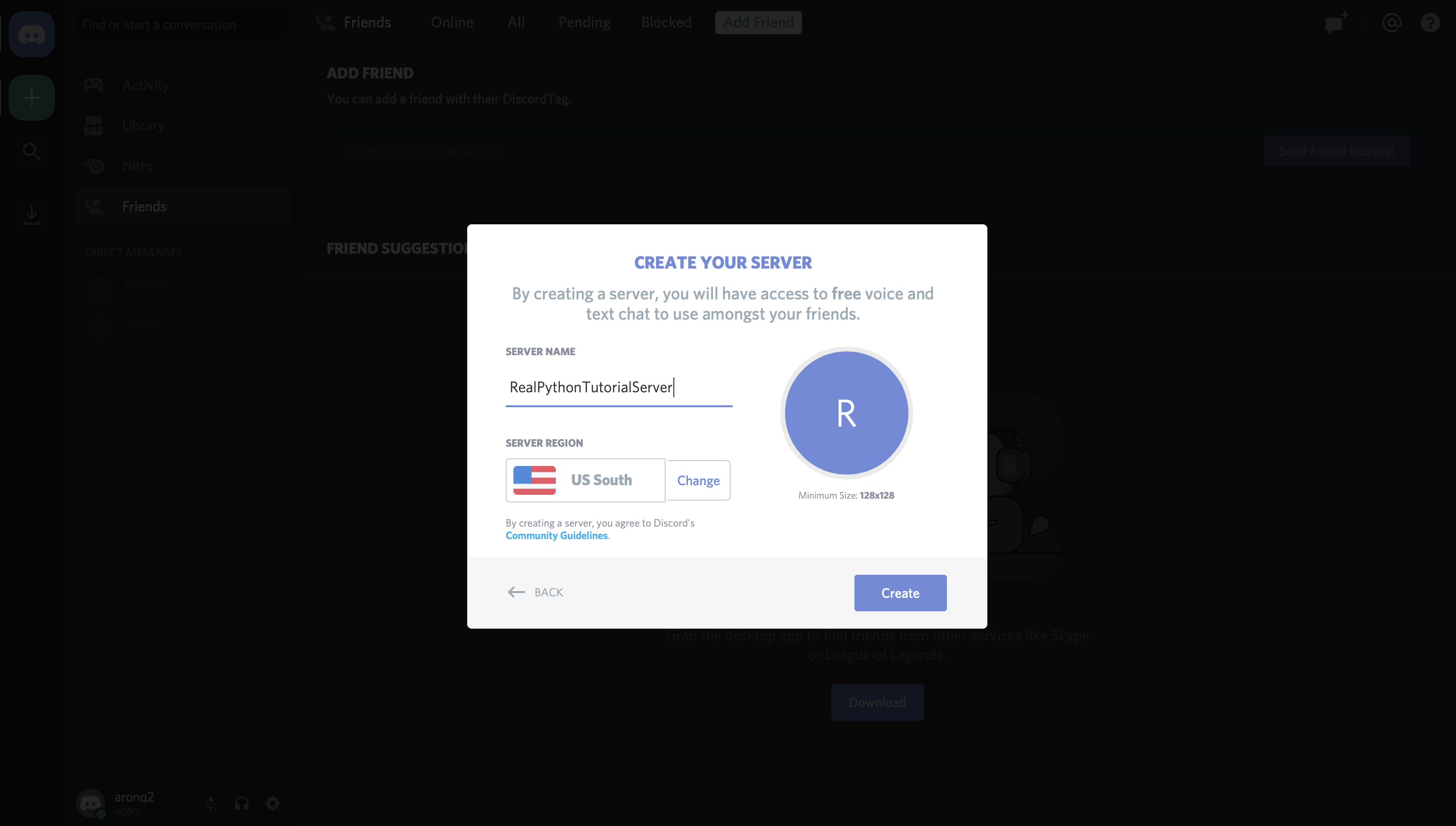
Once you’ve finished creating your guild, you’ll be able to see the users on the right-hand side and the channels on the left:
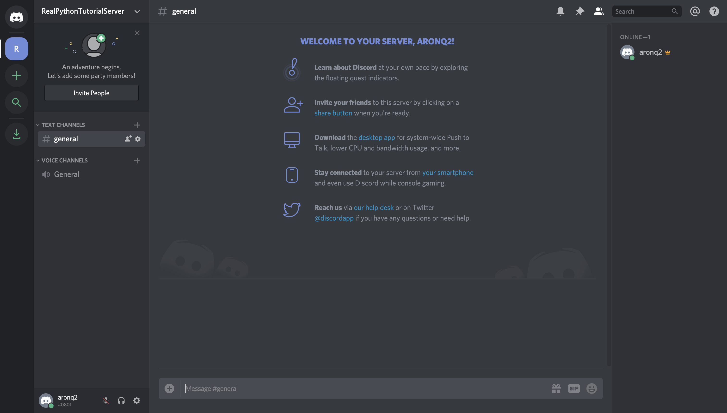
The final step on Discord is to register your bot with your new guild.
A bot can’t accept invites like a normal user can. Instead, you’ll add your bot using the OAuth2 protocol.
Technical Detail: OAuth2 is a protocol for dealing with authorization, where a service can grant a client application limited access based on the application’s credentials and allowed scopes.
To do so, head back to the Developer Portal and select the OAuth2 page from the left-hand navigation:
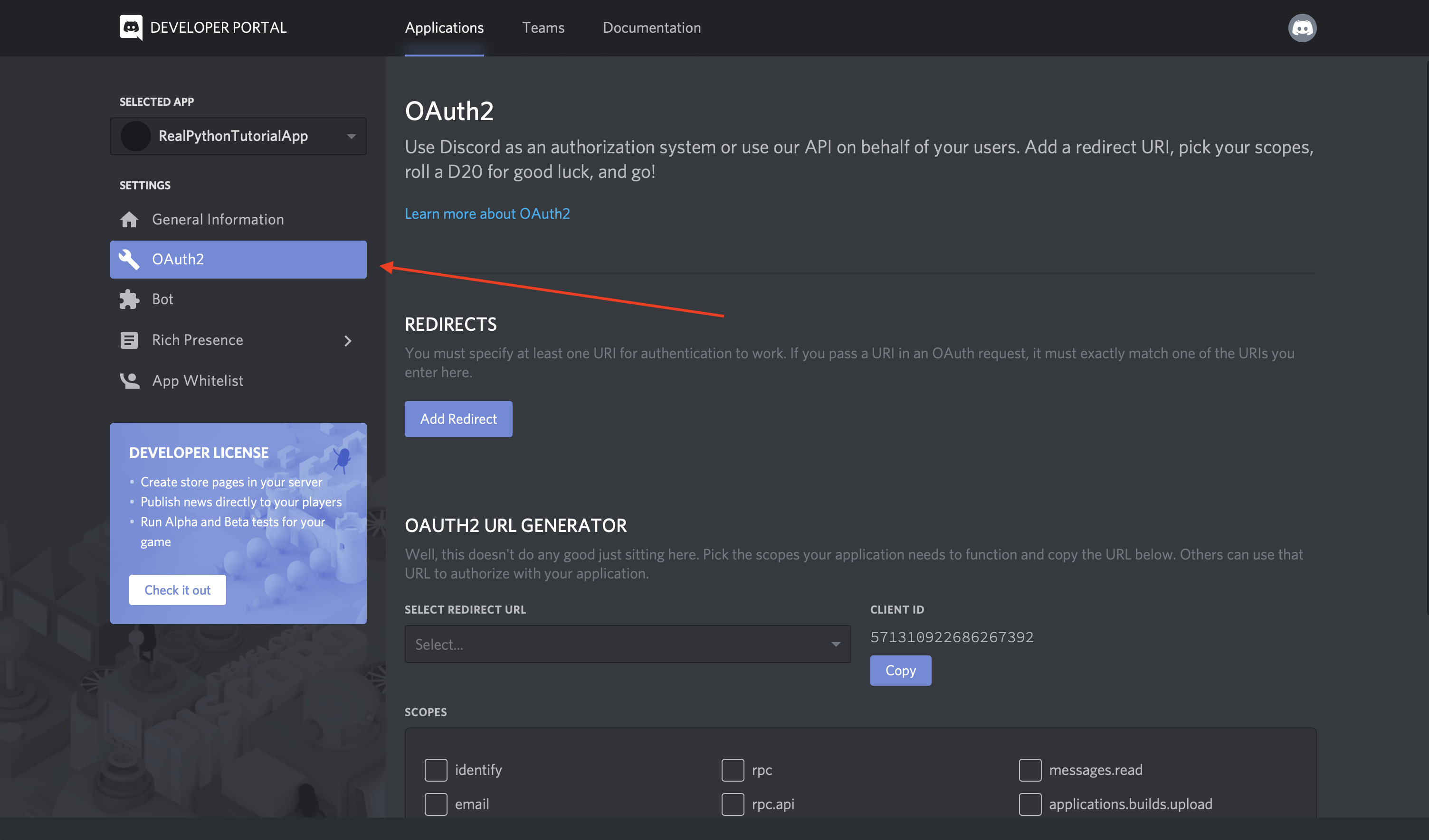
From this window, you’ll see the OAuth2 URL Generator.
This tool generates an authorization URL that hits Discord’s OAuth2 API and authorizes API access using your application’s credentials.
In this case, you’ll want to grant your application’s bot user access to Discord APIs using your application’s OAuth2 credentials.
To do this, scroll down and select bot from the SCOPES options and Administrator from BOT PERMISSIONS:
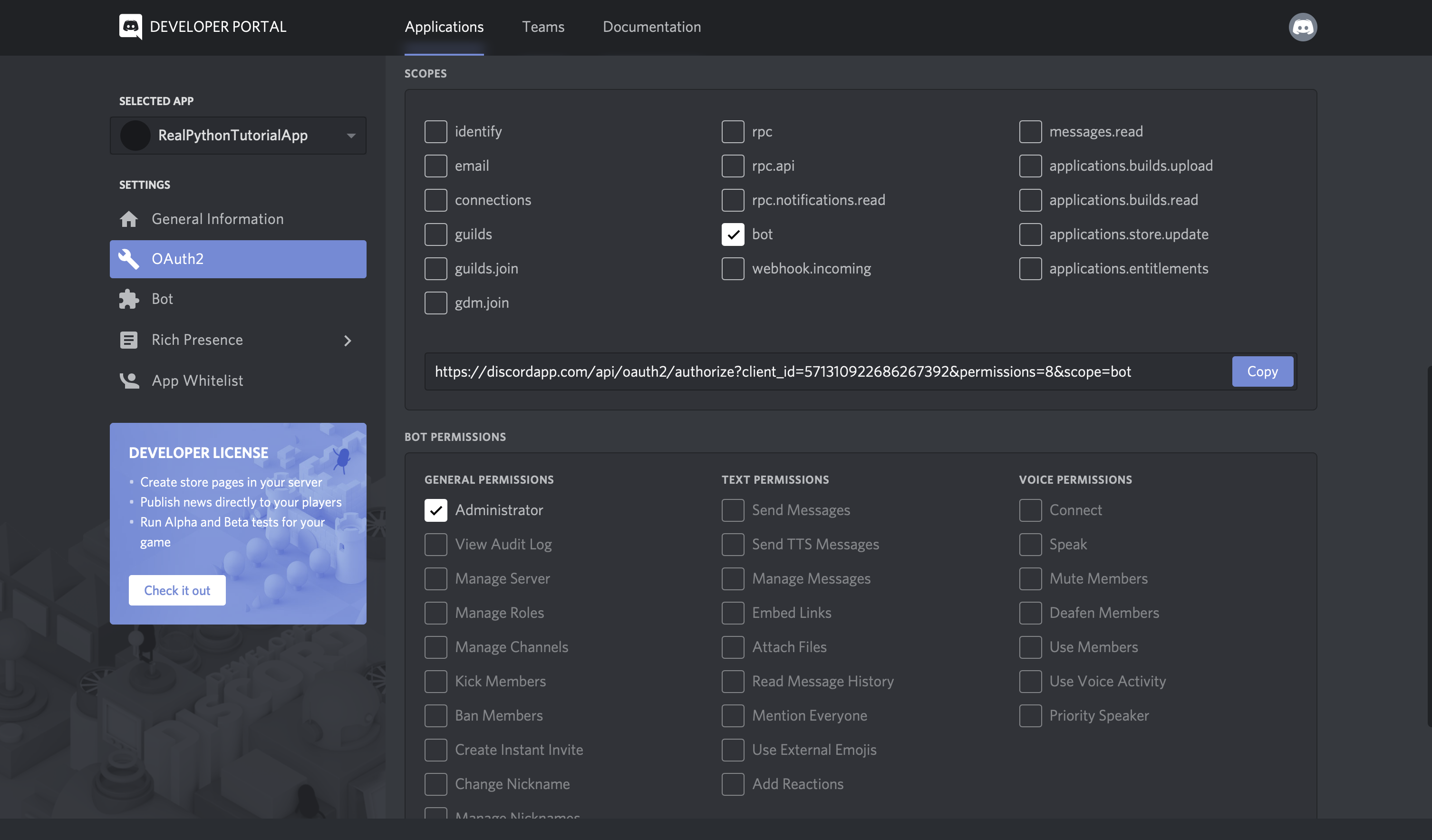
Now, Discord has generated your application’s authorization URL with the selected scope and permissions.
Disclaimer: While we’re using Administrator for the purposes of this tutorial, you should be as granular as possible when granting permissions in a real-world application.
Select Copy beside the URL that was generated for you, paste it into your browser, and select your guild from the dropdown options:
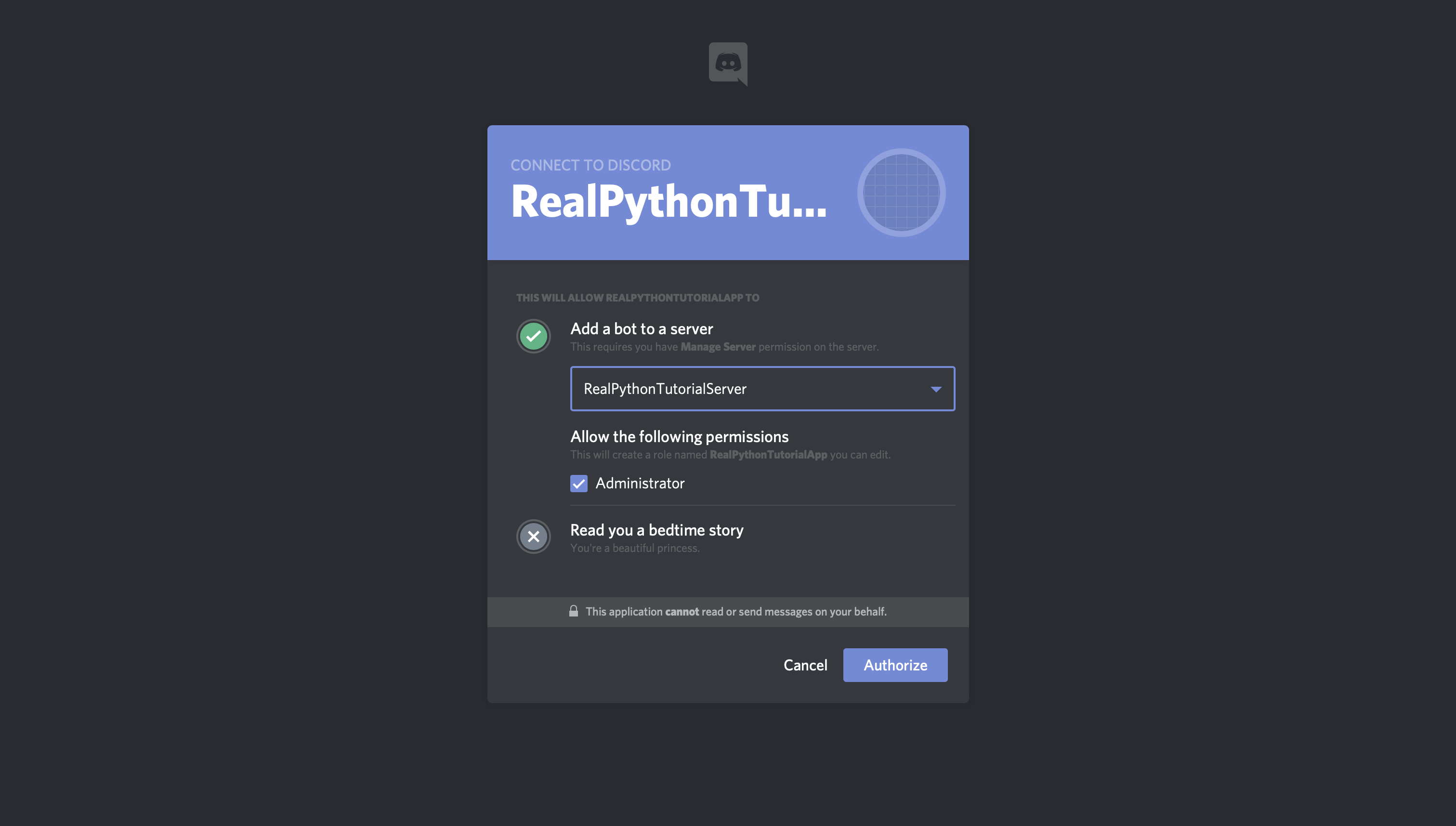
Click Authorize, and you’re done!
Note: You might get a reCAPTCHA before moving on. If so, you’ll need to prove you’re a human.
If you go back to your guild, then you’ll see that the bot has been added:
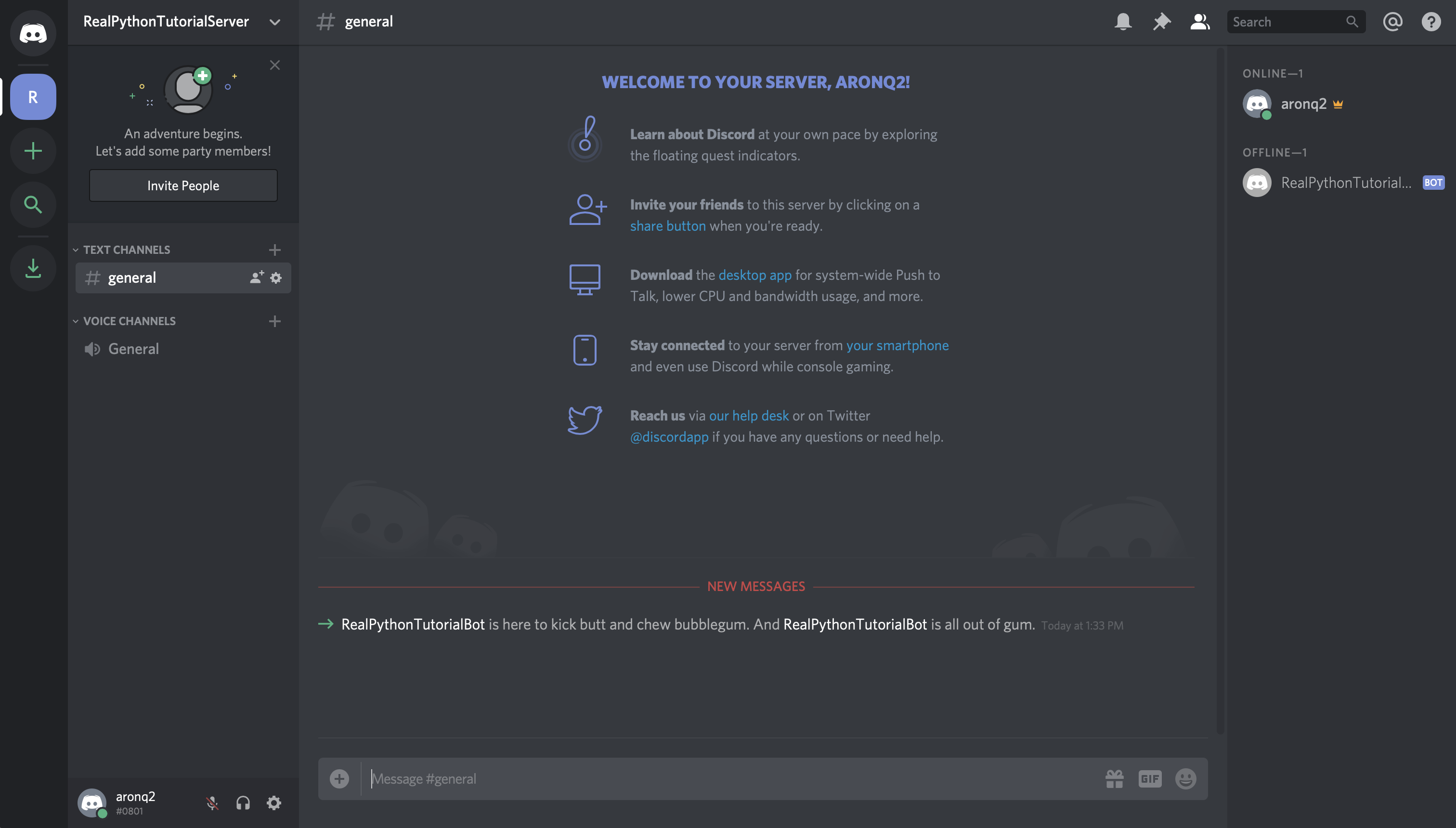
In summary, you’ve created:
Now, you know how to make a Discord bot using the Developer Portal. Next comes the fun stuff: implementing your bot in Python!
Since you’re learning how to make a Discord bot with Python, you’ll be using discord.py.
discord.py is a Python library that exhaustively implements Discord’s APIs in an efficient and Pythonic way. This includes utilizing Python’s implementation of Async IO.
Begin by installing discord.py with pip:
$ pip install -U discord.py
Now that you’ve installed discord.py, you’ll use it to create your first connection to Discord!
The first step in implementing your bot user is to create a connection to Discord. With discord.py, you do this by creating an instance of Client:
# bot.py
import os
import discord
from dotenv import load_dotenv
load_dotenv()
token = os.getenv('DISCORD_TOKEN')
client = discord.Client()
@client.event
async def on_ready():
print(f'{client.user} has connected to Discord!')
client.run(token)
A Client is an object that represents a connection to Discord. A Client handles events, tracks state, and generally interacts with Discord APIs.
Here, you’ve created a Client and implemented its on_ready() event handler, which handles the event when the Client has established a connection to Discord and it has finished preparing the data that Discord has sent, such as login state, guild and channel data, and more.
In other words, on_ready() will be called (and your message will be printed) once client is ready for further action. You’ll learn more about event handlers later in this article.
When you’re working with secrets such as your Discord token, it’s good practice to read it into your program from an environment variable. Using environment variables helps you:
While you could export DISCORD_TOKEN={your-bot-token}, an easier solution is to save a .env file on all machines that will be running this code. This is not only easier, since you won’t have to export your token every time you clear your shell, but it also protects you from storing your secrets in your shell’s history.
Create a file named .env in the same directory as bot.py:
# .env
DISCORD_TOKEN={your-bot-token}
You’ll need to replace {your-bot-token} with your bot’s token, which you can get by going back to the Bot page on the Developer Portal and clicking Copy under the TOKEN section:
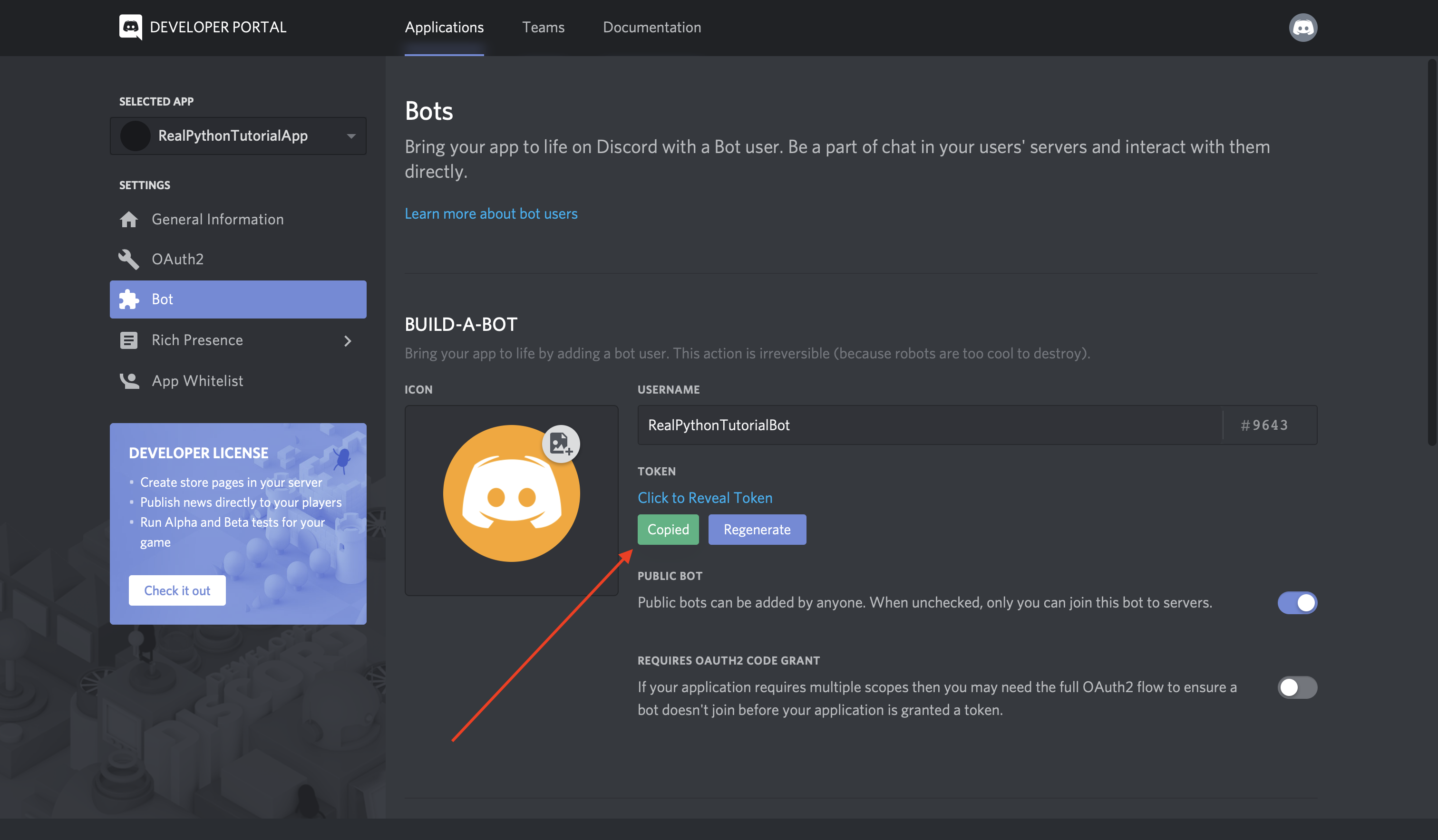
Looking back at the bot.py code, you’ll notice a library called dotenv. This library is handy for working with .env files. load_dotenv() loads environment variables from a .env file into your shell’s environment variables so that you can use them in your code.
Install dotenv with pip:
$ pip install -U python-dotenv
Finally, client.run() runs your Client using your bot’s token.
Now that you’ve set up both bot.py and .env, you can run your code:
$ python bot.py
RealPythonTutorialBot#9643 has connected to Discord!
Great! Your Client has connected to Discord using your bot’s token. In the next section, you’ll build on this Client by interacting with more Discord APIs.
Using a Client, you have access to a wide range of Discord APIs.
For example, let’s say you wanted to write the name and identifier of the guild that you registered your bot user with to the console.
First, you’ll need to add a new environment variable:
# .env
DISCORD_TOKEN={your-bot-token}
DISCORD_GUILD={your-guild-name}
Don’t forget that you’ll need to replace the two placeholders with actual values:
{your-bot-token}{your-guild-name}Remember that Discord calls on_ready(), which you used before, once the Client has made the connection and prepared the data. So, you can rely on the guild data being available inside on_ready():
# bot.py
import os
import discord
from dotenv import load_dotenv
load_dotenv()
TOKEN = os.getenv('DISCORD_TOKEN')
GUILD = os.getenv('DISCORD_GUILD')
client = discord.Client()
@client.event
async def on_ready():
for guild in client.guilds:
if guild.name == GUILD:
break
print(
f'{client.user} is connected to the following guild:\n'
f'{guild.name}(id: {guild.id})'
)
client.run(TOKEN)
Here, you looped through the guild data that Discord has sent client, namely client.guilds. Then, you found the guild with the matching name and printed a formatted string to stdout.
Note: Even though you can be pretty confident at this point in the tutorial that your bot is only connected to a single guild (so client.guilds[0] would be simpler), it’s important to realize that a bot user can be connected to many guilds.
Therefore, a more robust solution is to loop through client.guilds to find the one you’re looking for.
Run the program to see the results:
$ python bot.py
RealPythonTutorialBot#9643 is connected to the following guild:
RealPythonTutorialServer(id: 571759877328732195)
Great! You can see the name of your bot, the name of your server, and the server’s identification number.
Another interesting bit of data you can pull from a guild is the list of users who are members of the guild:
# bot.py
import os
import discord
from dotenv import load_dotenv
load_dotenv()
TOKEN = os.getenv('DISCORD_TOKEN')
GUILD = os.getenv('DISCORD_GUILD')
client = discord.Client()
@client.event
async def on_ready():
for guild in client.guilds:
if guild.name == GUILD:
break
print(
f'{client.user} is connected to the following guild:\n'
f'{guild.name}(id: {guild.id})\n'
)
members = '\n - '.join([member.name for member in guild.members])
print(f'Guild Members:\n - {members}')
client.run(TOKEN)
By looping through guild.members, you pulled the names of all of the members of the guild and printed them with a formatted string.
When you run the program, you should see at least the name of the account you created the guild with and the name of the bot user itself:
$ python bot.py
RealPythonTutorialBot#9643 is connected to the following guild:
RealPythonTutorialServer(id: 571759877328732195)
Guild Members:
- aronq2
- RealPythonTutorialBot
These examples barely scratch the surface of the APIs available on Discord, be sure to check out their documentation to see all that they have to offer.
Next, you’ll learn about some utility functions and how they can simplify these examples.
Let’s take another look at the example from the last section where you printed the name and identifier of the bot’s guild:
# bot.py
import os
import discord
from dotenv import load_dotenv
load_dotenv()
TOKEN = os.getenv('DISCORD_TOKEN')
GUILD = os.getenv('DISCORD_GUILD')
client = discord.Client()
@client.event
async def on_ready():
for guild in client.guilds:
if guild.name == GUILD:
break
print(
f'{client.user} is connected to the following guild:\n'
f'{guild.name}(id: {guild.id})'
)
client.run(TOKEN)
You could clean up this code by using some of the utility functions available in discord.py.
discord.utils.find() is one utility that can improve the simplicity and readability of this code by replacing the for loop with an intuitive, abstracted function:
# bot.py
import os
import discord
from dotenv import load_dotenv
load_dotenv()
TOKEN = os.getenv('DISCORD_TOKEN')
GUILD = os.getenv('DISCORD_GUILD')
client = discord.Client()
@client.event
async def on_ready():
guild = discord.utils.find(lambda g: g.name == GUILD, client.guilds)
print(
f'{client.user} is connected to the following guild:\n'
f'{guild.name}(id: {guild.id})'
)
client.run(TOKEN)
find() takes a function, called a predicate, which identifies some characteristic of the element in the iterable that you’re looking for. Here, you used a particular type of anonymous function, called a lambda, as the predicate.
In this case, you’re trying to find the guild with the same name as the one you stored in the DISCORD_GUILD environment variable. Once find() locates an element in the iterable that satisfies the predicate, it will return the element. This is essentially equivalent to the break statement in the previous example, but cleaner.
discord.py has even abstracted this concept one step further with the get() utility:
# bot.py
import os
import discord
from dotenv import load_dotenv
load_dotenv()
TOKEN = os.getenv('DISCORD_TOKEN')
GUILD = os.getenv('DISCORD_GUILD')
client = discord.Client()
@client.event
async def on_ready():
guild = discord.utils.get(client.guilds, name=GUILD)
print(
f'{client.user} is connected to the following guild:\n'
f'{guild.name}(id: {guild.id})'
)
client.run(TOKEN)
get() takes the iterable and some keyword arguments. The keyword arguments represent attributes of the elements in the iterable that must all be satisfied for get() to return the element.
In this example, you’ve identified name=GUILD as the attribute that must be satisfied.
Technical Detail: Under the hood, get() actually uses the attrs keyword arguments to build a predicate, which it then uses to call find().
Now that you’ve learned the basics of interacting with APIs, you’ll dive a little deeper into the function that you’ve been using to access them: on_ready().
You already learned that on_ready() is an event. In fact, you might have noticed that it is identified as such in the code by the client.event decorator.
But what is an event?
An event is something that happens on Discord that you can use to trigger a reaction in your code. Your code will listen for and then respond to events.
Using the example you’ve seen already, the on_ready() event handler handles the event that the Client has made a connection to Discord and prepared its response data.
So, when Discord fires an event, discord.py will route the event data to the corresponding event handler on your connected Client.
There are two ways in discord.py to implement an event handler:
client.event decoratorClient and overriding its handler methodsYou already saw the implementation using the decorator. Next, take a look at how to subclass Client:
# bot.py
import os
import discord
from dotenv import load_dotenv
load_dotenv()
token = os.getenv('DISCORD_TOKEN')
class CustomClient(discord.Client):
async def on_ready(self):
print(f'{self.user} has connected to Discord!')
client = CustomClient()
client.run(token)
Here, just like before, you’ve created a client variable and called .run() with your Discord token. The actual Client is different, however. Instead of using the normal base class, client is an instance of CustomClient, which has an overridden on_ready() function.
There is no difference between the two implementation styles of events, but this tutorial will primarily use the decorator version because it looks similar to how you implement Bot commands, which is a topic you’ll cover in a bit.
Technical Detail: Regardless of how you implement your event handler, one thing must be consistent: all event handlers in discord.py must be coroutines.
Now that you’ve learned how to create an event handler, let’s walk through some different examples of handlers you can create.
Previously, you saw the example of responding to the event where a member joins a guild. In that example, your bot user could send them a message, welcoming them to your Discord community.
Now, you’ll implement that behavior in your Client, using event handlers, and verify its behavior in Discord:
# bot.py
import os
import discord
from dotenv import load_dotenv
load_dotenv()
token = os.getenv('DISCORD_TOKEN')
client = discord.Client()
@client.event
async def on_ready():
print(f'{client.user.name} has connected to Discord!')
@client.event
async def on_member_join(member):
await member.create_dm()
await member.dm_channel.send(
f'Hi {member.name}, welcome to my Discord server!'
)
client.run(token)
Like before, you handled the on_ready() event by printing the bot user’s name in a formatted string. New, however, is the implementation of the on_member_join() event handler.
on_member_join(), as its name suggests, handles the event of a new member joining a guild.
In this example, you used member.create_dm() to create a direct message channel. Then, you used that channel to .send() a direct message to that new member.
Technical Detail: Notice the await keyword before member.create_dm() and member.dm_channel.send().
await suspends the execution of the surrounding coroutine until the execution of each coroutine has finished.
Now, let’s test out your bot’s new behavior.
First, run your new version of bot.py and wait for the on_ready() event to fire, logging your message to stdout:
$ python bot.py
RealPythonTutorialBot has connected to Discord!
Now, head over to Discord, log in, and navigate to your guild by selecting it from the left-hand side of the screen:
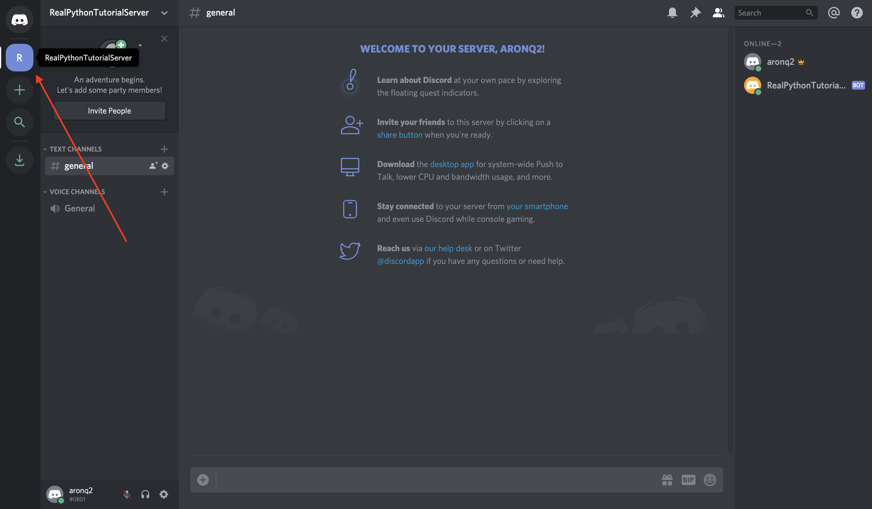
Select Invite People just beside the guild list where you selected your guild. Check the box that says Set this link to never expire and copy the link:
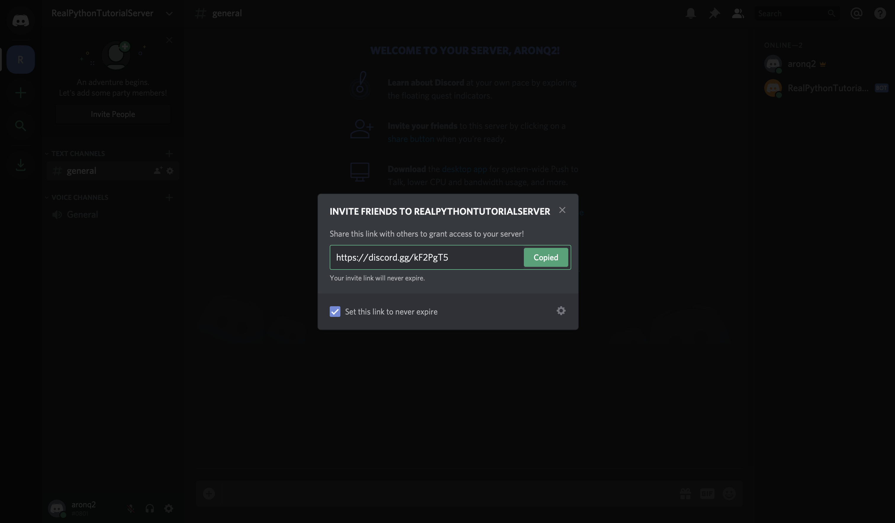
Now, with the invite link copied, create a new account and join the guild using your invite link:

First, you’ll see that Discord introduced you to the guild by default with an automated message. More importantly though, notice the badge on the left-hand side of the screen that notifies you of a new message:
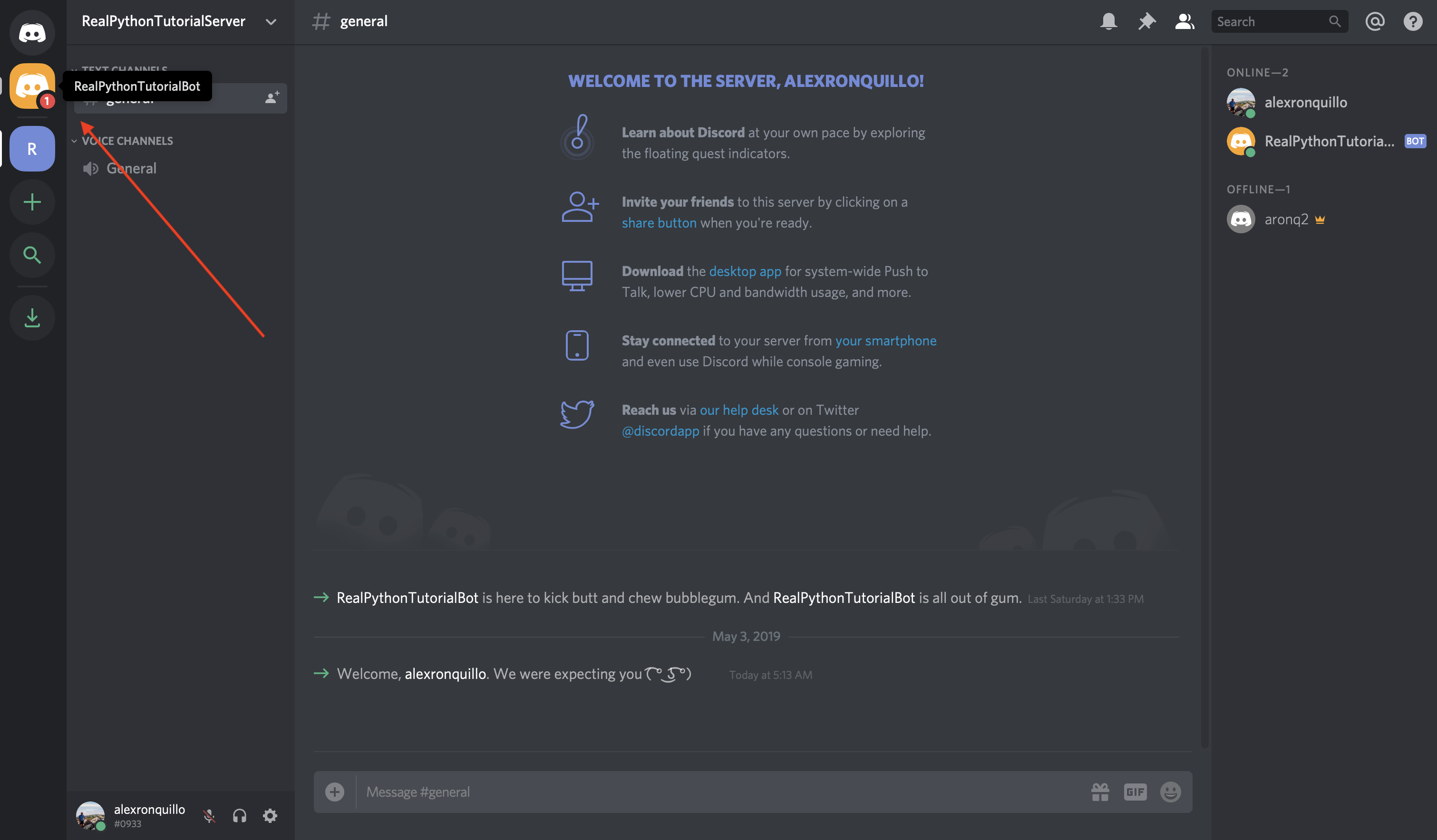
When you select it, you’ll see a private message from your bot user:
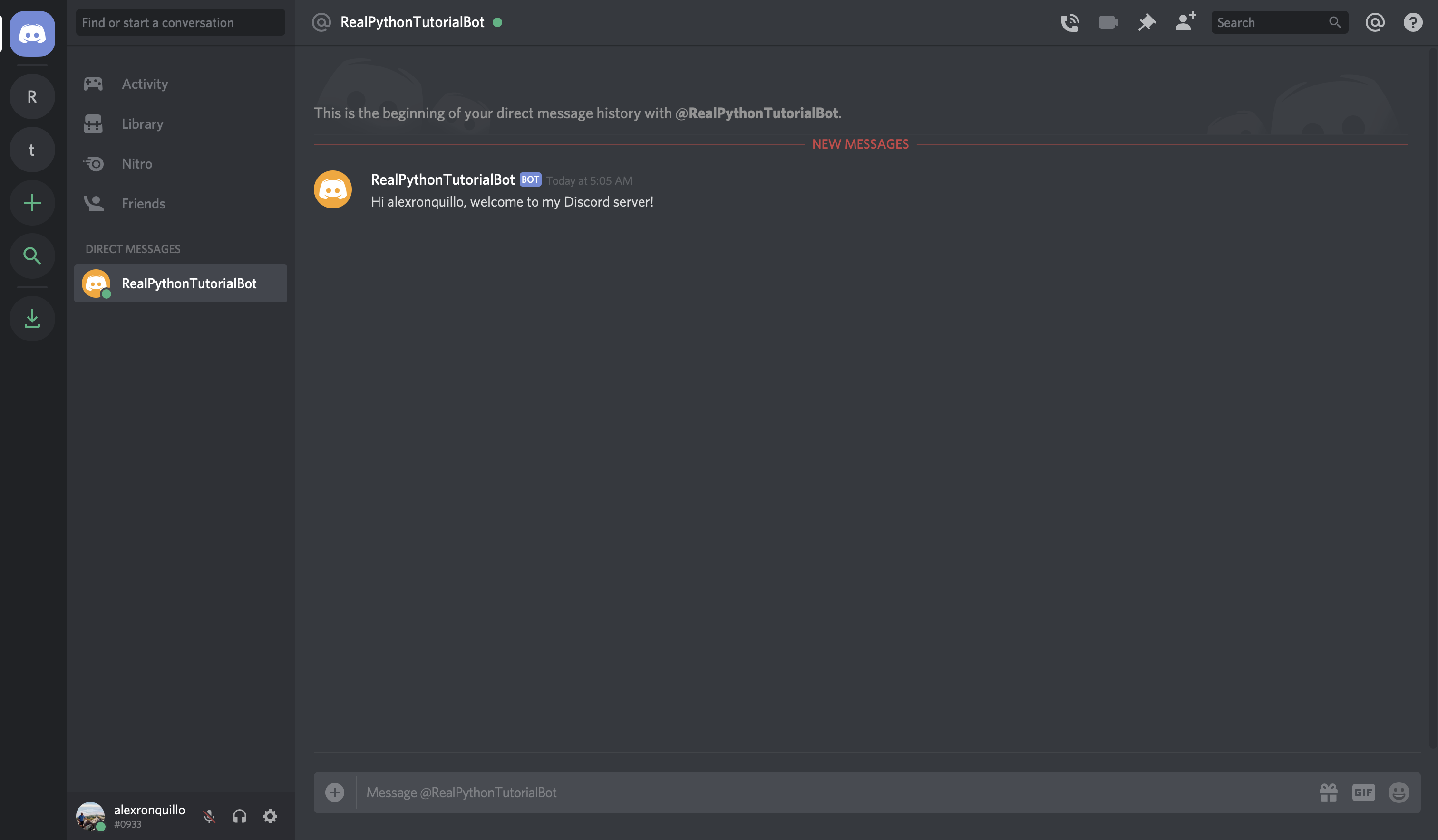
Perfect! Your bot user is now interacting with other users with minimal code.
Next, you’ll learn how to respond to specific user messages in the chat.
Let’s add on to the previous functionality of your bot by handling the on_message() event.
on_message() occurs when a message is posted in a channel that your bot has access to. In this example, you’ll respond to the message '99!' with a one-liner from the television show Brooklyn Nine-Nine:
@client.event
async def on_message(message):
if message.author == client.user:
return
brooklyn_99_quotes = [
'I\'m the human form of the 💯 emoji.',
'Bingpot!',
(
'Cool. Cool cool cool cool cool cool cool, '
'no doubt no doubt no doubt no doubt.'
),
]
if message.content == '99!':
response = random.choice(brooklyn_99_quotes)
await message.channel.send(response)
The bulk of this event handler looks at the message.content, checks to see if it’s equal to '99!', and responds by sending a random quote to the message’s channel if it is.
The other piece is an important one:
if message.author == client.user:
return
Because a Client can’t tell the difference between a bot user and a normal user account, your on_message() handler should protect against a potentially recursive case where the bot sends a message that it might, itself, handle.
To illustrate, let’s say you want your bot to listen for users telling each other 'Happy Birthday'. You could implement your on_message() handler like this:
@client.event
async def on_message(message):
if 'happy birthday' in message.content.lower():
await message.channel.send('Happy Birthday! 🎈🎉')
Aside from the potentially spammy nature of this event handler, it also has a devastating side effect. The message that the bot responds with contains the same message it’s going to handle!
So, if one person in the channel tells another “Happy Birthday,” then the bot will also chime in… again… and again… and again:
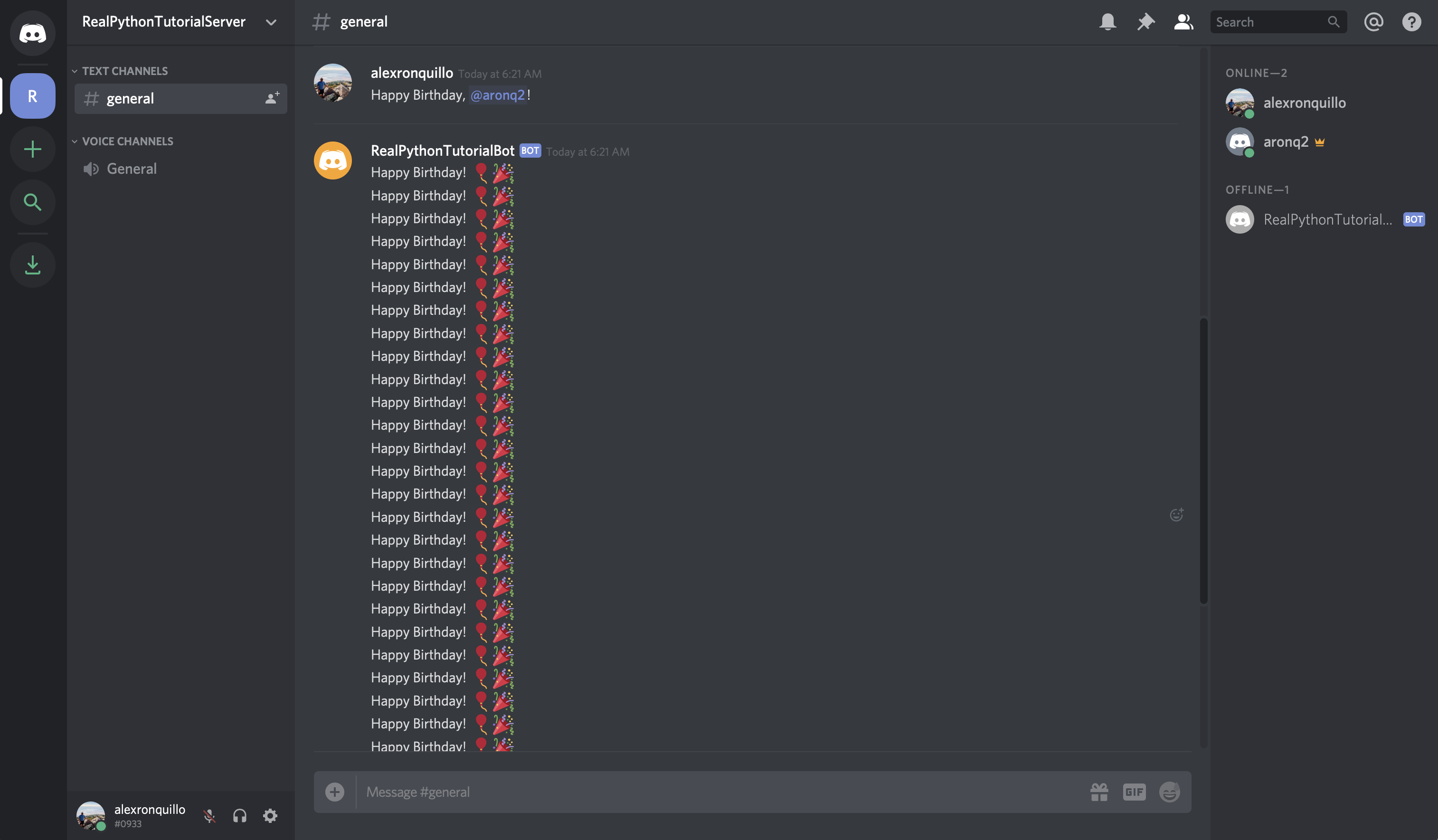
That’s why it’s important to compare the message.author to the client.user (your bot user), and ignore any of its own messages.
So, let’s fix bot.py:
# bot.py
import os
import random
import discord
from dotenv import load_dotenv
load_dotenv()
token = os.getenv('DISCORD_TOKEN')
client = discord.Client()
@client.event
async def on_ready():
print(f'{client.user.name} has connected to Discord!')
@client.event
async def on_member_join(member):
await member.create_dm()
await member.dm_channel.send(
f'Hi {member.name}, welcome to my Discord server!'
)
@client.event
async def on_message(message):
if message.author == client.user:
return
brooklyn_99_quotes = [
'I\'m the human form of the 💯 emoji.',
'Bingpot!',
(
'Cool. Cool cool cool cool cool cool cool, '
'no doubt no doubt no doubt no doubt.'
),
]
if message.content == '99!':
response = random.choice(brooklyn_99_quotes)
await message.channel.send(response)
client.run(token)
Don’t forget to import random at the top of the module, since the on_message() handler utilizes random.choice().
Run the program:
$ python bot.py
RealPythonTutorialBot has connected to Discord!
Finally, head over to Discord to test it out:
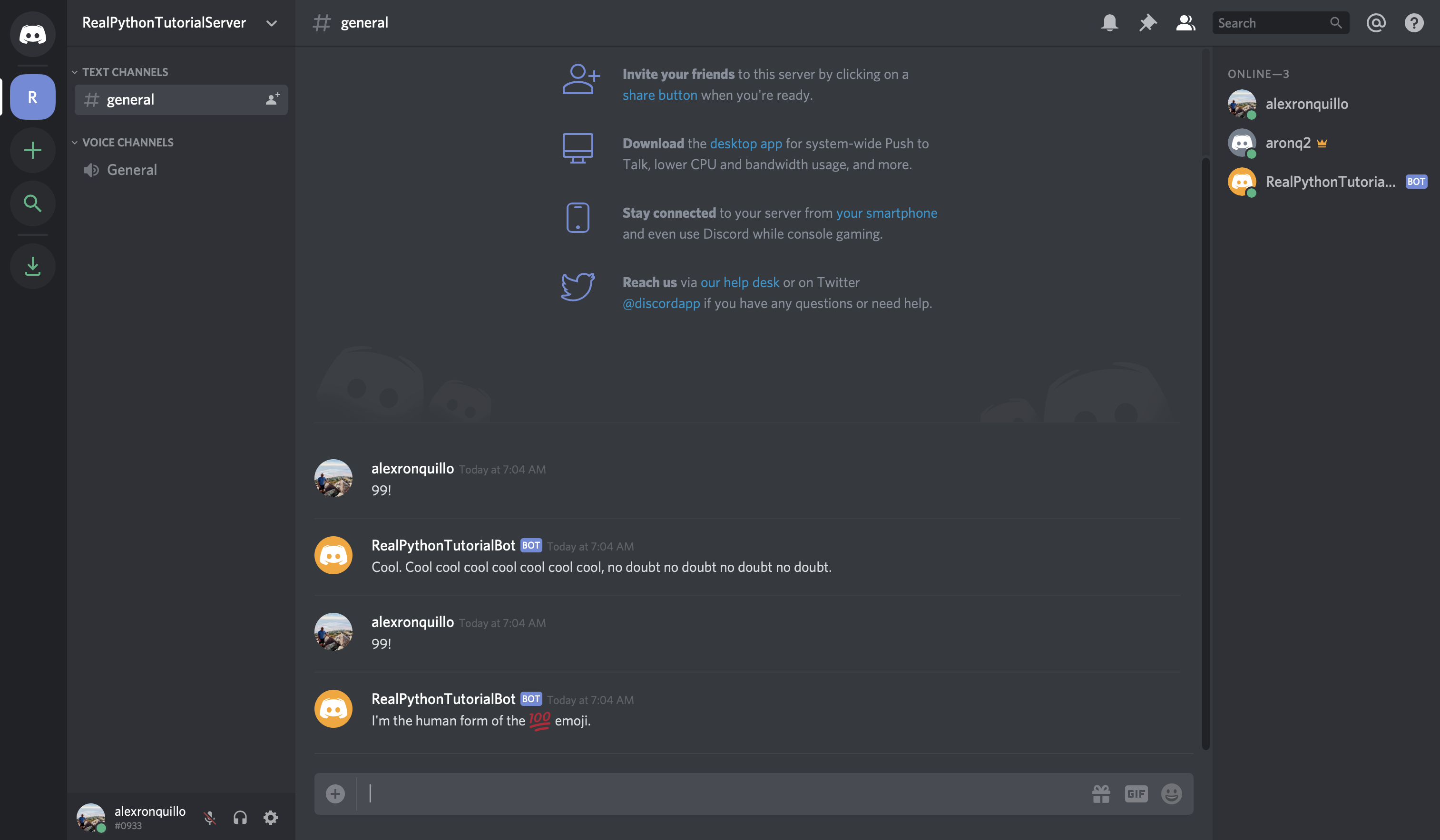
Great! Now that you’ve seen a few different ways to handle some common Discord events, you’ll learn how to deal with errors that event handlers may raise.
As you’ve seen already, discord.py is an event-driven system. This focus on events extends even to exceptions. When one event handler raises an Exception, Discord calls on_error().
The default behavior of on_error() is to write the error message and stack trace to stderr. To test this, add a special message handler to on_message():
# bot.py
import os
import random
import discord
from dotenv import load_dotenv
load_dotenv()
token = os.getenv('DISCORD_TOKEN')
client = discord.Client()
@client.event
async def on_ready():
print(f'{client.user.name} has connected to Discord!')
@client.event
async def on_member_join(member):
await member.create_dm()
await member.dm_channel.send(
f'Hi {member.name}, welcome to my Discord server!'
)
@client.event
async def on_message(message):
if message.author == client.user:
return
brooklyn_99_quotes = [
'I\'m the human form of the 💯 emoji.',
'Bingpot!',
(
'Cool. Cool cool cool cool cool cool cool, '
'no doubt no doubt no doubt no doubt.'
),
]
if message.content == '99!':
response = random.choice(brooklyn_99_quotes)
await message.channel.send(response)
elif message.content == 'raise-exception':
raise discord.DiscordException
client.run(token)
The new raise-exception message handler allows you to raise a DiscordException on command.
Run the program and type raise-exception into the Discord channel:
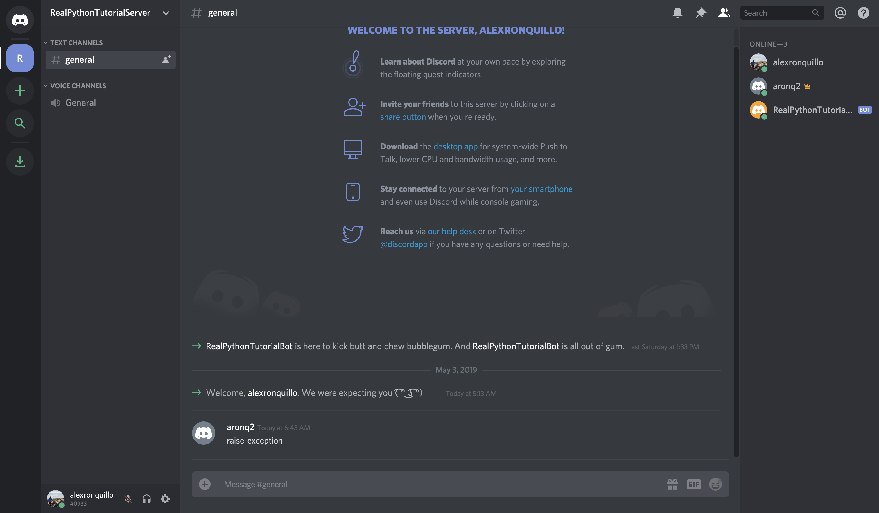
You should now see the Exception that was raised by your on_message() handler in the console:
$ python bot.py
RealPythonTutorialBot has connected to Discord!
Ignoring exception in on_message
Traceback (most recent call last):
File "/Users/alex.ronquillo/.pyenv/versions/discord-venv/lib/python3.7/site-packages/discord/client.py", line 255, in _run_event
await coro(*args, **kwargs)
File "bot.py", line 42, in on_message
raise discord.DiscordException
discord.errors.DiscordException
The exception was caught by the default error handler, so the output contains the message Ignoring exception in on_message. Let’s fix that by handling that particular error. To do so, you’ll catch the DiscordException and write it to a file instead.
The on_error() event handler takes the event as the first argument. In this case, we expect the event to be 'on_message'. It also accepts *args and **kwargs as flexible, positional and keyword arguments passed to the original event handler.
So, since on_message() takes a single argument, message, we expect args[0] to be the message that the user sent in the Discord channel:
@client.event
async def on_error(event, *args, **kwargs):
with open('err.log', 'a') as f:
if event == 'on_message':
f.write(f'Unhandled message: {args[0]}\n')
else:
raise
If the Exception originated in the on_message() event handler, you .write() a formatted string to the file err.log. If another event raises an Exception, then we simply want our handler to re-raise the exception to invoke the default behavior.
Run bot.py and send the raise-exception message again to view the output in err.log:
$ cat err.log
Unhandled message: <Message id=573845548923224084 pinned=False author=<Member id=543612676807327754 name='alexronquillo' discriminator='0933' bot=False nick=None guild=<Guild id=571759877328732195 name='RealPythonTutorialServer' chunked=True>>>
Instead of only a stack trace, you have a more informative error, showing the message that caused on_message() to raise the DiscordException, saved to a file for longer persistence.
Technical Detail: If you want to take the actual Exception into account when you’re writing your error messages to err.log, then you can use functions from sys, such as exc_info().
Now that you have some experience handling different events and interacting with Discord APIs, you’ll learn about a subclass of Client called Bot, which implements some handy, bot-specific functionality.
A Bot is a subclass of Client that adds a little bit of extra functionality that is useful when you’re creating bot users. For example, a Bot can handle events and commands, invoke validation checks, and more.
Before you get into the features specific to Bot, convert bot.py to use a Bot instead of a Client:
# bot.py
import os
import random
from dotenv import load_dotenv
# 1
from discord.ext import commands
load_dotenv()
token = os.getenv('DISCORD_TOKEN')
# 2
bot = commands.Bot(command_prefix='!')
@bot.event
async def on_ready():
print(f'{bot.user.name} has connected to Discord!')
bot.run(token)
As you can see, Bot can handle events the same way that Client does. However, notice the differences between Client and Bot:
Bot is imported from the discord.ext.commands module.Bot initializer requires a command_prefix, which you’ll learn more about in the next section.The extensions library, ext, offers several interesting components to help you create a Discord Bot. One such component is the Command.
Bot CommandsIn general terms, a command is an order that a user gives to a bot so that it will do something. Commands are different from events because they are:
In technical terms, a Command is an object that wraps a function that is invoked by a text command in Discord. The text command must start with the command_prefix, defined by the Bot object.
Let’s take a look at an old event to better understand what this looks like:
# bot.py
import os
import random
import discord
from dotenv import load_dotenv
load_dotenv()
TOKEN = os.getenv('DISCORD_TOKEN')
client = discord.Client()
@client.event
async def on_message(message):
if message.author == client.user:
return
brooklyn_99_quotes = [
'I\'m the human form of the 💯 emoji.',
'Bingpot!',
(
'Cool. Cool cool cool cool cool cool cool, '
'no doubt no doubt no doubt no doubt.'
),
]
if message.content == '99!':
response = random.choice(brooklyn_99_quotes)
await message.channel.send(response)
client.run(TOKEN)
Here, you created an on_message() event handler, which receives the message string and compares it to a pre-defined option: '99!'.
Using a Command, you can convert this example to be more specific:
# bot.py
import os
import random
from discord.ext import commands
from dotenv import load_dotenv
load_dotenv()
token = os.getenv('DISCORD_TOKEN')
bot = commands.Bot(command_prefix='!')
@bot.command(name='99')
async def nine_nine(ctx):
brooklyn_99_quotes = [
'I\'m the human form of the 💯 emoji.',
'Bingpot!',
(
'Cool. Cool cool cool cool cool cool cool, '
'no doubt no doubt no doubt no doubt.'
),
]
response = random.choice(brooklyn_99_quotes)
await ctx.send(response)
bot.run(token)
There are several important characteristics to understand about using Command:
Instead of using bot.event like before, you use bot.command(), passing the invocation command (name) as its argument.
The function will now only be called when !99 is mentioned in chat. This is different than the on_message() event, which was executed any time a user sent a message, regardless of the content.
The command must be prefixed with the exclamation point (! ) because that’s the command_prefix that you defined in the initializer for your Bot.
Any Command function (technically called a callback) must accept at least one parameter, called ctx, which is the Context surrounding the invoked Command.
A Context holds data such as the channel and guild that the user called the Command from.
Run the program:
$ python bot.py
With your bot running, you can now head to Discord to try out your new command:
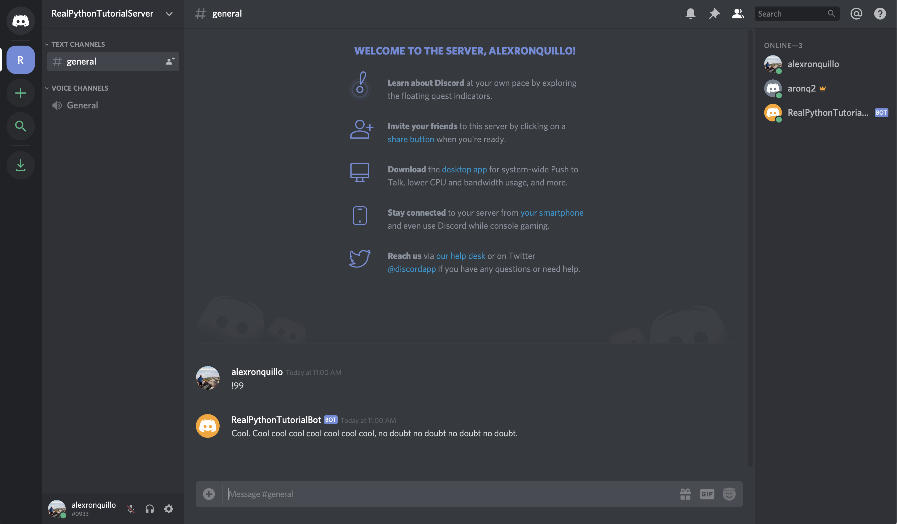
From the user’s point of view, the practical difference is that the prefix helps formalize the command, rather than simply reacting to a particular on_message() event.
This comes with other great benefits as well. For example, you can invoke the help command to see all the commands that your Bot handles:
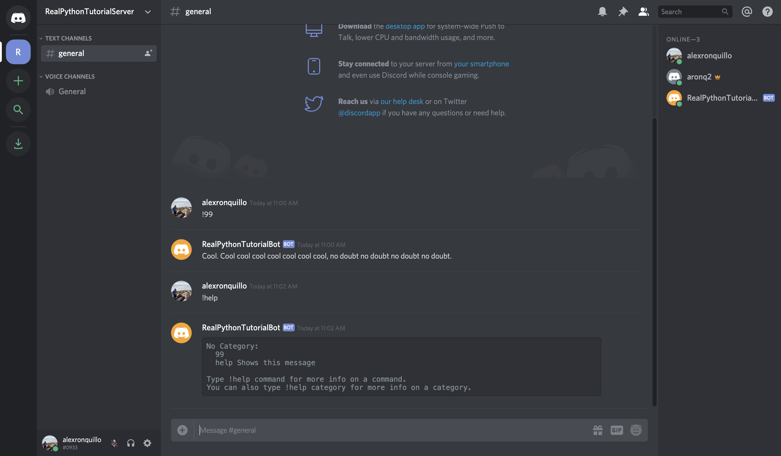
If you want to add a description to your command so that the help message is more informative, simply pass a help description to the .command() decorator:
# bot.py
import os
import random
from discord.ext import commands
from dotenv import load_dotenv
load_dotenv()
token = os.getenv('DISCORD_TOKEN')
bot = commands.Bot(command_prefix='!')
@bot.command(name='99', help='Responds with a random quote from Brooklyn 99')
async def nine_nine(ctx):
brooklyn_99_quotes = [
'I\'m the human form of the 💯 emoji.',
'Bingpot!',
(
'Cool. Cool cool cool cool cool cool cool, '
'no doubt no doubt no doubt no doubt.'
),
]
response = random.choice(brooklyn_99_quotes)
await ctx.send(response)
bot.run(token)
Now, when the user invokes the help command, your bot will present a description of your command:
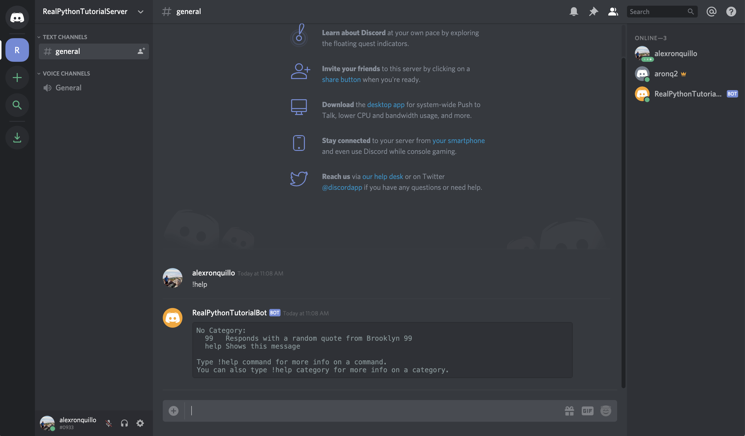
Keep in mind that all of this functionality exists only for the Bot subclass, not the Client superclass.
Command has another useful functionality: the ability to use a Converter to change the types of its arguments.
Another benefit of using commands is the ability to convert parameters.
Sometimes, you require a parameter to be a certain type, but arguments to a Command function are, by default, strings. A Converter lets you convert those parameters to the type that you expect.
For example, if you want to build a Command for your bot user to simulate rolling some dice (knowing what you’ve learned so far), you might define it like this:
@bot.command(name='roll_dice', help='Simulates rolling dice.')
async def roll(ctx, number_of_dice, number_of_sides):
dice = [
str(random.choice(range(1, number_of_sides + 1)))
for _ in range(number_of_dice)
]
await ctx.send(', '.join(dice))
You defined roll to take two parameters:
Then, you decorated it with .command() so that you can invoke it with the !roll_dice command. Finally, you .send() the results in a message back to the channel.
While this looks correct, it isn’t. Unfortunately, if you run bot.py, and invoke the !roll_dice command in your Discord channel, you’ll see the following error:
$ python bot.py
Ignoring exception in command roll_dice:
Traceback (most recent call last):
File "/Users/alex.ronquillo/.pyenv/versions/discord-venv/lib/python3.7/site-packages/discord/ext/commands/core.py", line 63, in wrapped
ret = await coro(*args, **kwargs)
File "bot.py", line 40, in roll
for _ in range(number_of_dice)
TypeError: 'str' object cannot be interpreted as an integer
The above exception was the direct cause of the following exception:
Traceback (most recent call last):
File "/Users/alex.ronquillo/.pyenv/versions/discord-venv/lib/python3.7/site-packages/discord/ext/commands/bot.py", line 860, in invoke
await ctx.command.invoke(ctx)
File "/Users/alex.ronquillo/.pyenv/versions/discord-venv/lib/python3.7/site-packages/discord/ext/commands/core.py", line 698, in invoke
await injected(*ctx.args, **ctx.kwargs)
File "/Users/alex.ronquillo/.pyenv/versions/discord-venv/lib/python3.7/site-packages/discord/ext/commands/core.py", line 72, in wrapped
raise CommandInvokeError(exc) from exc
discord.ext.commands.errors.CommandInvokeError: Command raised an exception: TypeError: 'str' object cannot be interpreted as an integer
In other words, range() can’t accept a str as an argument. Instead, it must be an int. While you could cast each value to an int, there is a better way: you can use a Converter .
In discord.py, a Converter is defined using Python 3’s function annotations:
@bot.command(name='roll_dice', help='Simulates rolling dice.')
async def roll(ctx, number_of_dice: int, number_of_sides: int):
dice = [
str(random.choice(range(1, number_of_sides + 1)))
for _ in range(number_of_dice)
]
await ctx.send(', '.join(dice))
You added : int annotations to the two parameters that you expect to be of type int. Try the command again:
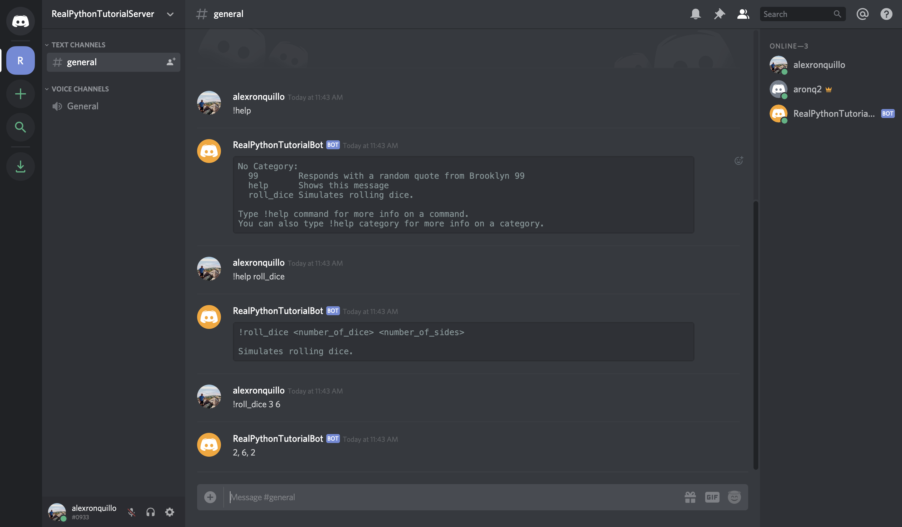
With that little change, your command works! The difference is that you’re now converting the command arguments to int, which makes them compatible with your function’s logic.
Note: A Converter can be any callable, not merely data types. The argument will be passed to the callable, and the return value will be passed into the Command.
Next, you’ll learn about the Check object and how it can improve your commands.
A Check is a predicate that is evaluated before a Command is executed to ensure that the Context surrounding the Command invocation is valid.
In an earlier example, you did something similar to verify that the user who sent a message that the bot handles was not the bot user, itself:
if message.author == client.user:
return
The commands extension provides a cleaner and more usable mechanism for performing this kind of check, namely using Check objects.
To demonstrate how this works, assume you want to support a command !create_channel <channel_name> that creates a new channel. However, you only want to allow administrators the ability to create new channels with this command.
First, you’ll need to create a new member role in the admin. Go into the Discord guild and select the {Server Name} → Server Settings menu:
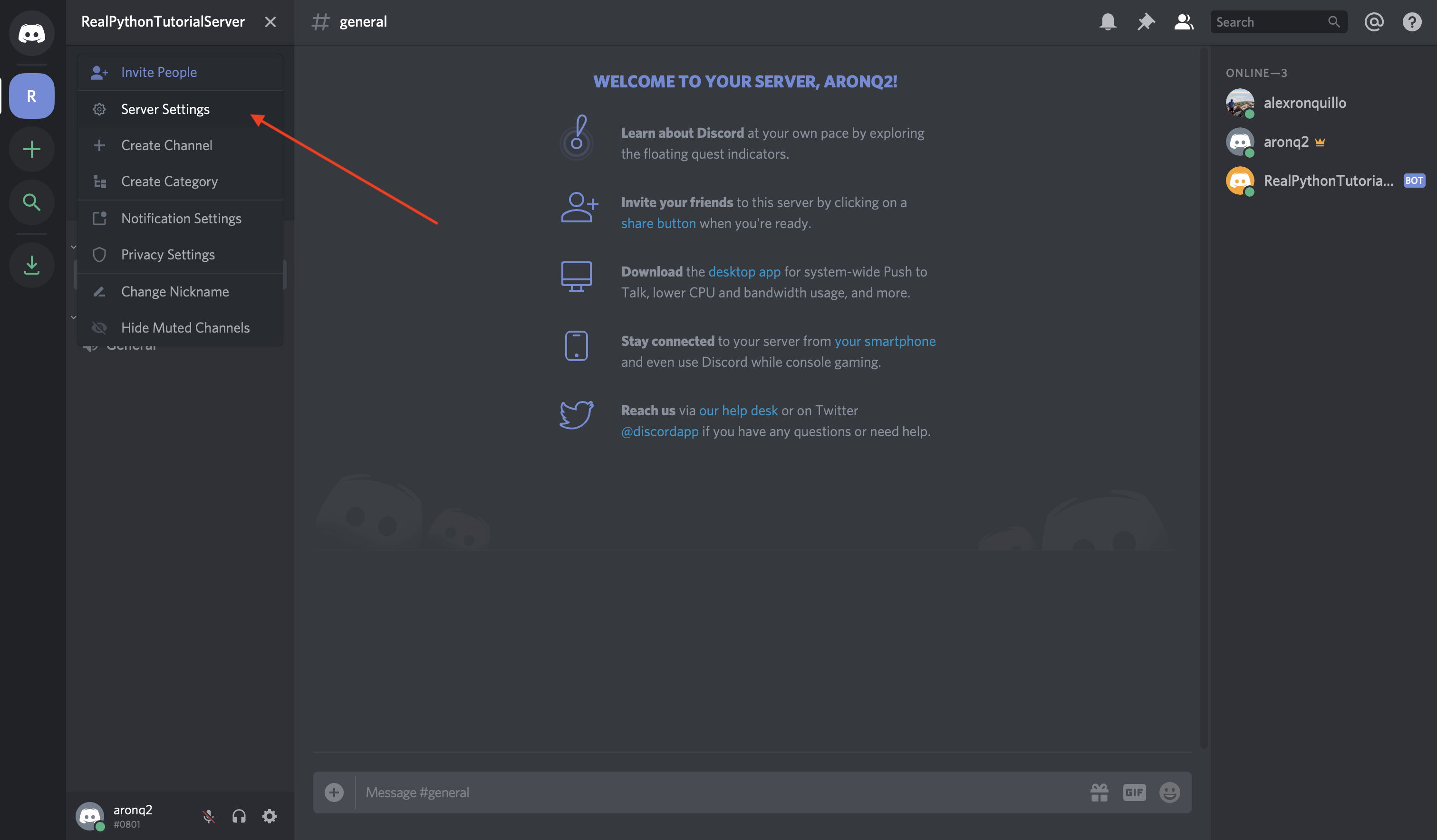
Then, select Roles from the left-hand navigation list:
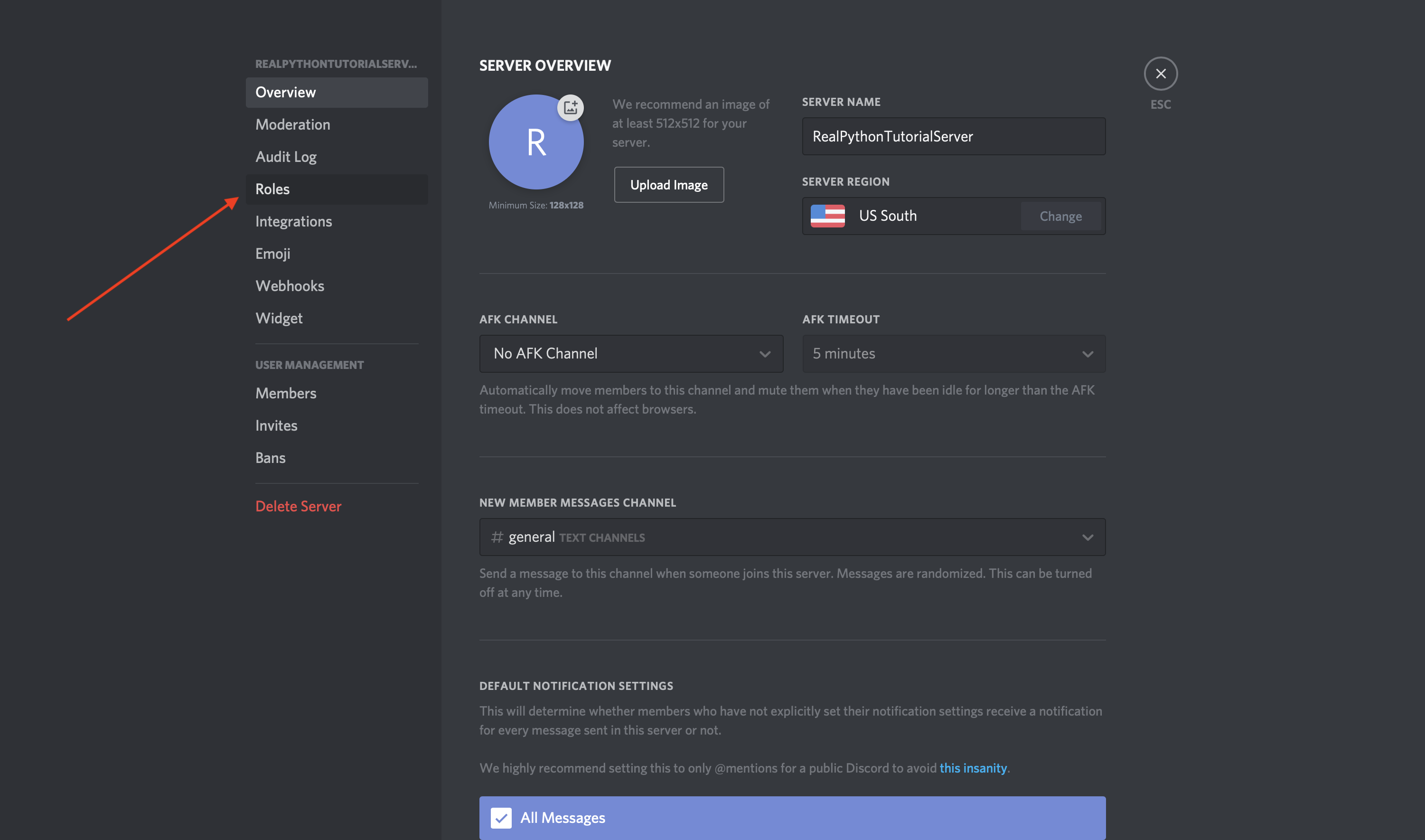
Finally select the + sign next to ROLES and enter the name admin and select Save Changes:
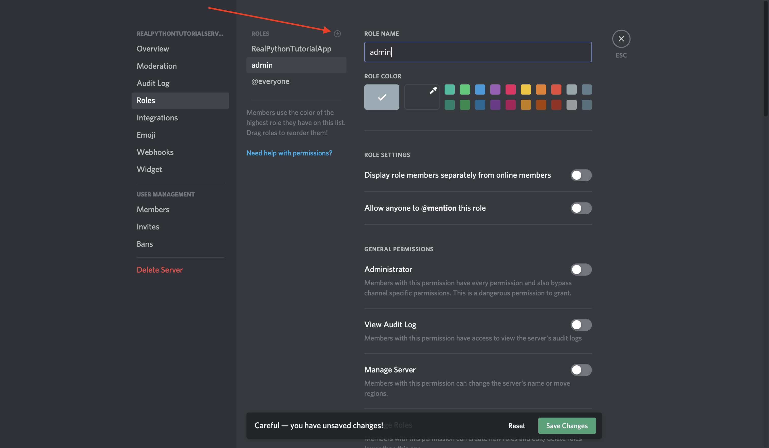
Now, you’ve created an admin role that you can assign to particular users. Next, you’ll update bot.py to Check the user’s role before allowing them to initiate the command:
# bot.py
import os
import discord
from discord.ext import commands
from dotenv import load_dotenv
load_dotenv()
TOKEN = os.getenv('DISCORD_TOKEN')
bot = commands.Bot(command_prefix='!')
@bot.command(name='create-channel')
@commands.has_role('admin')
async def create_channel(ctx, channel_name='real-python'):
guild = ctx.guild
existing_channel = discord.utils.get(guild.channels, name=channel_name)
if not existing_channel:
print(f'Creating a new channel: {channel_name}')
await guild.create_text_channel(channel_name)
bot.run(TOKEN)
In bot.py, you have a new Command function, called create_channel() which takes an optional channel_name and creates that channel. create_channel() is also decorated with a Check called has_role().
You also use discord.utils.get() to ensure that you don’t create a channel with the same name as an existing channel.
If you run this program as it is and type !create-channel into your Discord channel, then you’ll see the following error message:
$ python bot.py
Ignoring exception in command create-channel:
Traceback (most recent call last):
File "/Users/alex.ronquillo/.pyenv/versions/discord-venv/lib/python3.7/site-packages/discord/ext/commands/bot.py", line 860, in invoke
await ctx.command.invoke(ctx)
File "/Users/alex.ronquillo/.pyenv/versions/discord-venv/lib/python3.7/site-packages/discord/ext/commands/core.py", line 691, in invoke
await self.prepare(ctx)
File "/Users/alex.ronquillo/.pyenv/versions/discord-venv/lib/python3.7/site-packages/discord/ext/commands/core.py", line 648, in prepare
await self._verify_checks(ctx)
File "/Users/alex.ronquillo/.pyenv/versions/discord-venv/lib/python3.7/site-packages/discord/ext/commands/core.py", line 598, in _verify_checks
raise CheckFailure('The check functions for command {0.qualified_name} failed.'.format(self))
discord.ext.commands.errors.CheckFailure: The check functions for command create-channel failed.
This CheckFailure says that has_role('admin') failed. Unfortunately, this error only prints to stdout. It would be better to report this to the user in the channel. To do so, add the following event:
@bot.event
async def on_command_error(ctx, error):
if isinstance(error, commands.errors.CheckFailure):
await ctx.send('You do not have the correct role for this command.')
This event handles an error event from the command and sends an informative error message back to the original Context of the invoked Command.
Try it all again, and you should see an error in the Discord channel:
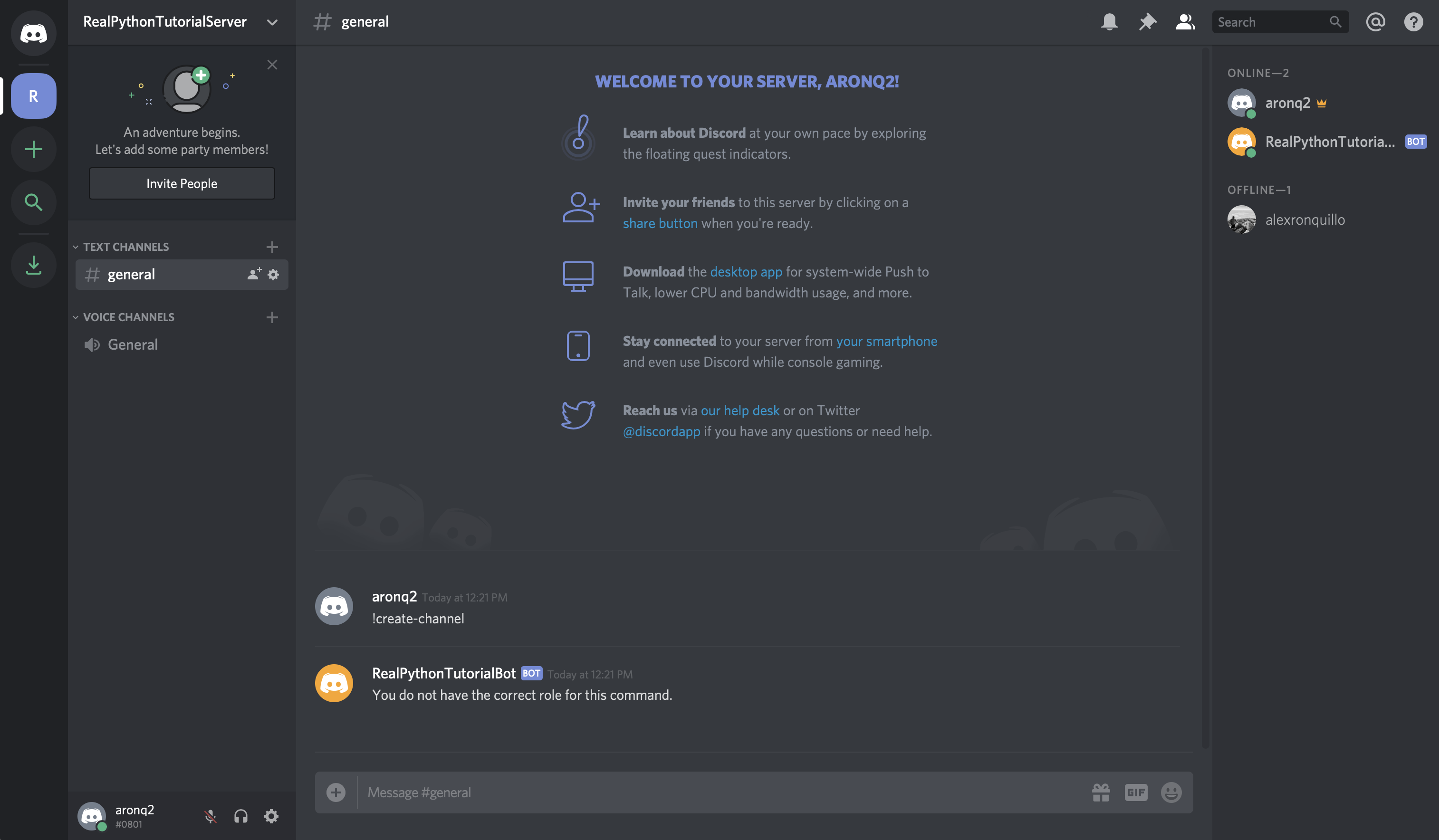
Great! Now, to resolve the issue, you’ll need to give yourself the admin role:
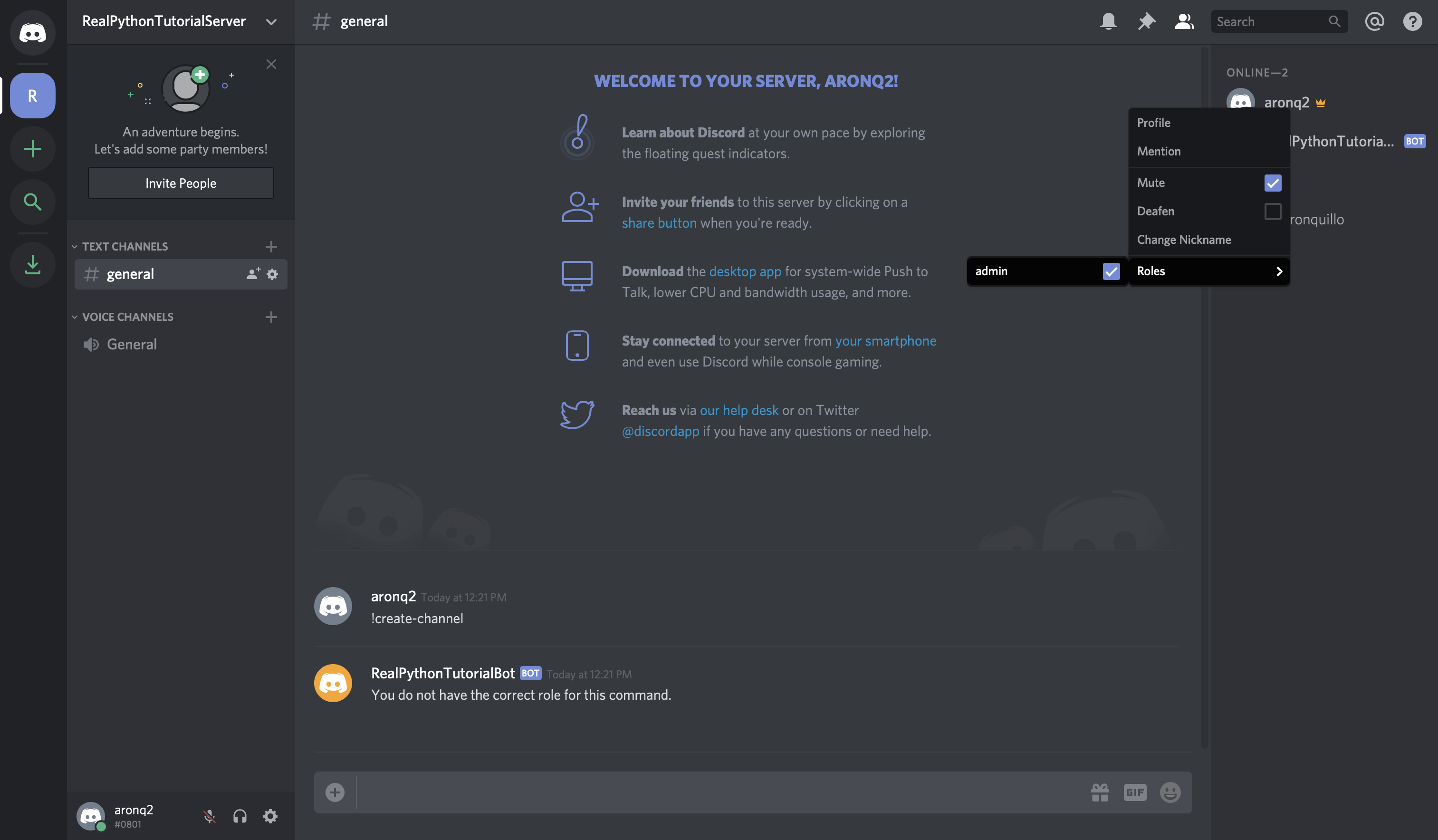
With the admin role, your user will pass the Check and will be able to create channels using the command.
Note: Keep in mind that in order to assign a role, your user will have to have the correct permissions. The easiest way to ensure this is to sign in with the user that you created the guild with.
When you type !create-channel again, you’ll successfully create the channel real-python:
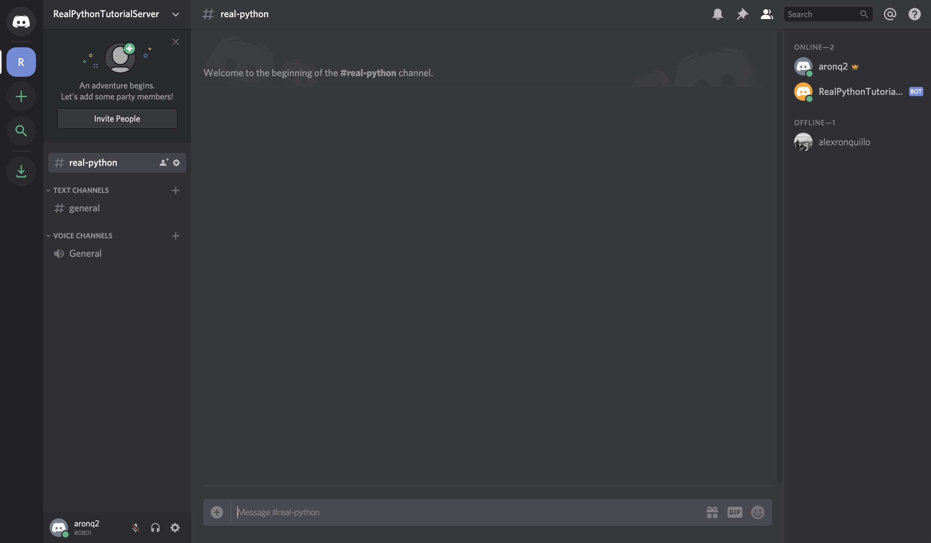
Also, note that you can pass the optional channel_name argument to name the channel to whatever you want!
With this last example, you combined a Command, an event, a Check, and even the get() utility to create a useful Discord bot!
Congratulations! Now, you’ve learned how to make a Discord bot in Python. You’re able to build bots for interacting with users in guilds that you create or even bots that other users can invite to interact with their communities. Your bots will be able to respond to messages and commands and numerous other events.
In this tutorial, you learned the basics of creating your own Discord bot. You now know:
discord.py is so valuableBot connectionTo read more about the powerful discord.py library and take your bots to the next level, read through their extensive documentation. Also, now that you’re familiar with Discord APIs in general, you have a better foundation for building other types of Discord applications.
[ Improve Your Python With 🐍 Python Tricks 💌 – Get a short & sweet Python Trick delivered to your inbox every couple of days. >> Click here to learn more and see examples ]
# datePublished: #Mon Aug 19 14:00:00 2019# dateUpdated: #Mon Aug 19 14:00:00 2019# # Person begin #################### name: #Real Python# # Person end ###################### # Item end ######################## # Item begin ###################### id: #https://realpython.com/effective-python-environment/# title: #An Effective Python Environment: Making Yourself at Home# link: #https://realpython.com/effective-python-environment/# description: #This guide will walk you through the decisions you need to make when customizing your development environment for working with Python.# content: #When you’re first learning a new programming language, a lot of your time and effort go into understanding the syntax, code style, and built-in tooling. This is just as true for Python as it is for any other language. Once you gain enough familiarity to be comfortable with the ins and outs of Python, you can start to invest time into building a Python environment that will foster your productivity.
Your shell is more than a prebuilt program provided to you as-is. It’s a framework on which you can build an ecosystem. This ecosystem will come to fit your needs so that you can spend less time fiddling and more time thinking about the next big project you’re working on.
Although no two developers have the same setup, there are a number of choices everyone faces when cultivating their Python environment. It’s important to understand each of these decisions and the options available to you!
By the end of this article, you’ll be able to answer questions like:
Once you’ve answered these questions for yourself, you can embark on the journey of creating a Python environment to call your very own. Let’s get started!
Free Bonus: Click here to get access to a free 5-day class that shows you how to avoid common dependency management issues with tools like Pip, PyPI, Virtualenv, and requirements files.
When you use a command-line interface (CLI), you execute commands and see their output. A shell is a program that provides this (usually text-based) interface to you. Shells often provide their own programming language that you can use to manipulate files, install software, and so on.
There are more unique shells than could be reasonably listed here, so you’ll see a few prominent ones. Others differ in syntax or enhanced features, but they generally provide the same core functionality.
Unix is a family of operating systems first developed in the early days of computing. Unix’s popularity has lasted through today, heavily inspiring Linux and macOS. The first shells were developed for use with Unix and Unix-like operating systems.
sh)The Bourne shell—developed by Stephen Bourne for Bell Labs in 1979—was one of the first to incorporate the idea of environment variables, conditionals, and loops. It has provided a strong basis for many other shells in use today and is still available on most systems at /bin/sh.
bash)Built on the success of the original Bourne shell, bash introduced improved user-interaction features. With bash, you get Tab completion, history, and wildcard searching for commands and paths. The bash programming language provides more data types, like arrays.
zsh)zsh combines many of the best features from other shells along with a few of its own tricks into one experience. zsh offers autocorrection of misspelled commands, shorthand for manipulating multiple files, and advanced options for customizing your command prompt.
zsh also provides a framework for deep customization. The Oh My Zsh project supplies a rich set of themes and plugins, and is often used hand in hand with zsh.
macOS will ship with zsh as its default shell starting with Catalina, speaking to the shell’s popularity. Consider acquainting yourself with zsh now so that you’ll be comfortable with it going forward.
If you’re feeling particularly adventurous, you can give Xonsh a try. Xonsh is a shell that combines some features of other Unix-like shells with the power of Python syntax. You can use the language you already know to accomplish tasks on your filesystem and so on.
Although Xonsh is powerful, it lacks the compatibility other shells tend to share. You might not be able to run many existing shell scripts in Xonsh as a result. If you find that you like Xonsh, but compatibility is a concern, then you can use Xonsh as a supplement to your activities in a more widely used shell.
Similarly to Unix-like operating systems, Windows also offers a number of options when it comes to shells. The shells offered in Windows vary in features and syntax, so you may need to try several to find one you like best.
cmd.exe)CMD (short for “command”) is the default CLI shell for Windows. It’s the successor to COMMAND.COM, the shell built for DOS (disk operating system).
Because DOS and Unix evolved independently, the commands and syntax in CMD are markedly different from shells built for Unix-like systems. However, CMD still provides the same core functionality for browsing and manipulating files, running commands, and viewing output.
PowerShell was released in 2006 and also ships with Windows. It provides Unix-like aliases for most commands, so if you’re coming to Windows from macOS or Linux or have to use both, then PowerShell might be great for you.
PowerShell is vastly more powerful than CMD. With PowerShell you can:
Microsoft has released a Windows subsystem for Linux (WSL) for running Linux directly on Windows. If you install WSL, then you can use zsh, bash, or any other Unix-like shell. If you want strong compatibility across your Windows and macOS or Linux environments, then be sure to give WSL a try. You may also consider dual-booting Linux and Windows as an alternative.
See this comparison of command shells for exhaustive coverage.
Early developers used terminals to interact with a central mainframe computer. These were devices with a keyboard and a screen or printer that would display computed output.
Today, computers are portable and don’t require separate devices to interact with them, but the terminology still remains. Whereas a shell provides the prompt and interpreter you use to interface with text-based CLI tools, a terminal emulator (often shortened to terminal) is the graphical application you run to access the shell.
Almost any terminal you encounter should support the same basic features:
The terminal options available for macOS are all full-featured, differing mostly in aesthetics and specific integrations with other tools.
If you’re using a Mac, then you may have used the built-in Terminal app before. Terminal supports all the usual functionality, and you can also customize the color scheme and a few hotkeys. It’s a nice enough tool if you don’t need many bells and whistles. You can find the Terminal app in Applications → Utilities → Terminal on macOS.
I’ve been a long-time user of iTerm2. It takes the developer experience on Mac a step further, offering a much wider palette of customization and productivity options that enable you to:
A Python API ships with the latest versions of iTerm2, so you can even improve your Python chops by developing more intricate customizations!
iTerm2 is popular enough to enjoy first-class integration with several other tools, and has a healthy community building plugins and so on. It’s a good choice because of its more frequent release cycle compared to Terminal, which only updates as often as macOS does.
A relative newcomer, Hyper is a terminal built on Electron, a framework for building desktop applications using web technologies. Electron apps are heavily customizable because they’re “just JavaScript” under the hood. You can create any functionality that you can write the JavaScript for.
On the other hand, JavaScript is a high-level programming language and won’t always perform as well as low-level languages like Objective-C or Swift. Be mindful of the plugins you install or create!
As with the shell options, Windows terminal options vary widely in utility. Some are tightly bound to a particular shell as well.
Command Prompt is the graphical application you can use to work with CMD in Windows. Like CMD, it’s a bare-bones tool for getting a few small things done. Although Command Prompt and CMD provide fewer features than other alternatives, you can be confident that they’ll be available on nearly every Windows installation and in a consistent place.
Cygwin is a third-party suite of tools for Windows that provides a Unix-like wrapper. This was my preferred setup when I was in Windows, but you may consider adopting the Windows Subsystem for Linux as it receives more traction and polish.
Microsoft recently released an open source terminal for Windows 10 called Windows Terminal. It lets you work in CMD, PowerShell, and even the Windows Subsystem for Linux. If you need to do a fair amount of shell work in Windows, then Windows Terminal is probably your best bet! Windows Terminal is still in late beta, so it doesn’t ship with Windows yet. Check the documentation for instructions on getting access.
With your choice of terminal and shell made, you can focus your attention on your Python environment specifically.
Something you’ll eventually run into is the need to run multiple versions of Python. Projects you use may only run on certain versions, or you may be interested in creating a project that supports multiple Python versions. You can configure your Python environment to accommodate these needs.
macOS and most Unix operating systems come with a version of Python installed by default. This is often called the system Python. The system Python works just fine, but it’s usually out of date. As of this writing, macOS High Sierra still ships with Python 2.7.10 as the system Python.
Note: You’ll almost certainly want to install the latest version of Python at a minimum, so you’ll have at least two versions of Python already.
It’s important that you leave the system Python as the default, because many parts of the system rely on the default Python being a specific version. This is one of many great reasons to customize your Python environment!
How do you navigate this? Tooling is here to help.
pyenvpyenv is a mature tool for installing and managing multiple Python versions on macOS. I recommend installing it with Homebrew. If you’re using Windows, you can use pyenv-win. After you’ve got pyenv installed, you can install multiple versions of Python into your Python environment with a few short commands:
$ pyenv versions
* system
$ python --version
Python 2.7.10
$ pyenv install 3.7.3 # This may take some time
$ pyenv versions
* system
3.7.3
You can manage which Python you’d like to use in your current session, globally, or on a per-project basis as well. pyenv will make the python command point to whichever Python you specify. Note that none of these overrides the default system Python for other applications, so you’re safe to use them however they work best for you within your Python environment:
$ pyenv global 3.7.3
$ pyenv versions
system
* 3.7.3 (set by /Users/dhillard/.pyenv/version)
$ pyenv local 3.7.3
$ pyenv versions
system
* 3.7.3 (set by /Users/dhillard/myproj/.python-version)
$ pyenv shell 3.7.3
$ pyenv versions
system
* 3.7.3 (set by PYENV_VERSION environment variable)
$ python --version
Python 3.7.3
Because I use a specific version of Python for work, the latest version of Python for personal projects, and multiple versions for testing open source projects, pyenv has proven to be a fairly smooth way for me to manage all these different versions within my own Python environment. See Managing Multiple Python Versions with pyenv for a detailed overview of the tool.
condaIf you’re in the data science community, you might already be using Anaconda (or Miniconda). Anaconda is a sort of one-stop shop for data science software that supports more than just Python.
If you don’t need the data science packages or all the things that come pre-packaged with Anaconda, pyenv might be a better lightweight solution for you. Managing Python versions is pretty similar in each, though. You can install Python versions similarly to pyenv, using the conda command:
$ conda install python=3.7.3
You’ll see a verbose list of all the dependent software conda will install, and it will ask you to confirm.
conda doesn’t have a way to set the “default” Python version or even a good way to see which versions of Python you’ve installed. Rather, it hinges on the concept of “environments,” which you can read more about in the following sections.
Now you know how to manage multiple Python versions. Often, you’ll be working on multiple projects that need the same Python version.
Because each project has its own set of dependencies, it’s a good practice to avoid mixing them. If all the dependencies are installed together in a single Python environment, then it will be difficult to discern where each one came from. In the worst cases, two different projects may depend on two different versions of a package, but with Python you can only have one version of a package installed at one time. What a mess!
Enter virtual environments. You can think of a virtual environment as a carbon copy of a base version of Python. If you’ve installed Python 3.7.3, for example, then you can create many virtual environments based off of it. When you install a package in a virtual environment, you do it in isolation from other Python environments you may have. Each virtual environment has its own copy of the python executable.
Tip: Most virtual environment tooling provides a way to update your shell’s command prompt to show the current active virtual environment. Make sure to do this if you frequently switch between projects so you’re sure you’re working inside the correct virtual environment.
venvvenv ships with Python versions 3.3+. You can create virtual environments just by passing it a path at which to store the environment’s python, installed packages, and so on:
$ python -m venv ~/.virtualenvs/my-env
You activate a virtual environment by sourcing its activate script:
$ source ~/.virtualenvs/my-env/bin/activate
You exit the virtual environment using the deactivate command, which is made available when you activate the virtual environment:
(my-env)$ deactivate
venv is built on the wonderful work and successes of the independent virtualenv project. virtualenv still provides a few interesting features of its own, but venv is nice because it provides the utility of virtual environments without requiring you to install additional software. You can probably get pretty far with it if you’re working mostly in a single Python version in your Python environment.
If you’re already managing multiple Python versions (or plan to), then it could make sense to integrate with that tooling to simplify the process of making new virtual environments with specific versions of Python. The pyenv and conda ecosystems both provide ways to specify the Python version to use when you create new virtual environments, covered in the following sections.
pyenv-virtualenvIf you’re using pyenv, then pyenv-virtualenv enhances pyenv with a subcommand for managing virtual environments:
// Create virtual environment
$ pyenv virtualenv 3.7.3 my-env
// Activate virtual environment
$ pyenv activate my-env
// Exit virtual environment
(my-env)$ pyenv deactivate
I switch contexts between a large handful of projects on a day-to-day basis. As a result, I have at least a dozen distinct virtual environments to manage in my Python environment. What’s really nice about pyenv-virtualenv is that you can configure a virtual environment using the pyenv local command and have pyenv-virtualenv auto-activate the right environments as you switch to different directories:
$ pyenv virtualenv 3.7.3 proj1
$ pyenv virtualenv 3.7.3 proj2
$ cd /Users/dhillard/proj1
$ pyenv local proj1
(proj1)$ cd ../proj2
$ pyenv local proj2
(proj2)$ pyenv versions
system
3.7.3
3.7.3/envs/proj1
3.7.3/envs/proj2
proj1
* proj2 (set by /Users/dhillard/proj2/.python-version)
pyenv and pyenv-virtualenv have provided a particularly fluid workflow in my Python environment.
condaYou saw earlier that conda treats environments, rather than Python versions, as the main method of working. conda has built-in support for managing virtual environments:
// Create virtual environment
$ conda create --name my-env python=3.7.3
// Activate virtual environment
$ conda activate my-env
// Exit virtual environment
(my-env)$ conda deactivate
conda will install the specified version of Python if it isn’t already installed, so you don’t have to run conda install python=3.7.3 first.
pipenvpipenv is a relatively new tool that seeks to combine package management (more on this in a moment) with virtual environment management. It mostly abstracts the virtual environment management from you, which can be great as long as things go smoothly:
$ cd /Users/dhillard/myproj
// Create virtual environment
$ pipenv install
Creating a virtualenv for this project…
Pipfile: /Users/dhillard/myproj/Pipfile
Using /path/to/pipenv/python3.7 (3.7.3) to create virtualenv…
✔ Successfully created virtual environment!
Virtualenv location: /Users/dhillard/.local/share/virtualenvs/myproj-nAbMEAt0
Creating a Pipfile for this project…
Pipfile.lock not found, creating…
Locking [dev-packages] dependencies…
Locking [packages] dependencies…
Updated Pipfile.lock (a65489)!
Installing dependencies from Pipfile.lock (a65489)…
🐍 ▉▉▉▉▉▉▉▉▉▉▉▉▉▉▉▉▉▉▉▉▉▉▉▉▉▉▉▉▉▉▉▉ 0/0 — 00:00:00
To activate this project's virtualenv, run pipenv shell.
Alternatively, run a command inside the virtualenv with pipenv run.
// Activate virtual environment (uses a subshell)
$ pipenv shell
Launching subshell in virtual environment…
. /Users/dhillard/.local/share/virtualenvs/test-nAbMEAt0/bin/activate
// Exit virtual environment (by exiting subshell)
(myproj-nAbMEAt0)$ exit
pipenv does all the heavy lifting of creating a virtual environment and activating it for you. If you look carefully, you can see that it also creates a file called Pipfile. After you first run pipenv install, this file contains just a few things:
[[source]]
name = "pypi"
url = "https://pypi.org/simple"
verify_ssl = true
[dev-packages]
[packages]
[requires]
python_version = "3.7"
In particular, note that it shows python_version = "3.7". By default, pipenv creates a virtual Python environment using the same Python version it was installed under. If you want to use a different Python version, then you can create the Pipfile yourself before running pipenv install and specify the version you want. If you have pyenv installed, then pipenv will use it to install the specified Python version if necessary.
Abstracting virtual environment management is a noble goal of pipenv, but it does get hung up with hard-to-read errors occasionally. Give it a try, but don’t worry if you feel confused or overwhelmed by it. The tool, documentation, and community will grow and improve around it as it matures.
To get an in-depth introduction to virtual environments, be sure to read Python Virtual Environments: A Primer.
For many of the projects you work on, you’ll probably need some number of third-party packages. Those packages may have their own dependencies in turn. In the early days of Python, using packages involved manually downloading files and pointing Python at them. Today, we’re fortunate to have a variety of package management tools available to us.
Most package managers work in tandem with virtual environments, isolating the packages you install in one Python environment from another. Using the two together is where you really start to see the power of the tools available to you.
pippip (pip installs packages) has been the de facto standard for package management in Python for several years. It was heavily inspired by an earlier tool called easy_install. Python incorporated pip into the standard distribution starting in version 3.4. pip automates the process of downloading packages and making Python aware of them.
If you have multiple virtual environments, then you can see that they’re isolated by installing a few packages in one:
$ pyenv virtualenv 3.7.3 proj1
$ pyenv activate proj1
(proj1)$ pip list
Package Version
---------- ---------
pip 19.1.1
setuptools 40.8.0
(proj1)$ python -m pip install requests
Collecting requests
Downloading .../requests-2.22.0-py2.py3-none-any.whl (57kB)
100% |████████████████████████████████| 61kB 2.2MB/s
Collecting chardet<3.1.0,>=3.0.2 (from requests)
Downloading .../chardet-3.0.4-py2.py3-none-any.whl (133kB)
100% |████████████████████████████████| 143kB 1.7MB/s
Collecting certifi>=2017.4.17 (from requests)
Downloading .../certifi-2019.6.16-py2.py3-none-any.whl (157kB)
100% |████████████████████████████████| 163kB 6.0MB/s
Collecting urllib3!=1.25.0,!=1.25.1,<1.26,>=1.21.1 (from requests)
Downloading .../urllib3-1.25.3-py2.py3-none-any.whl (150kB)
100% |████████████████████████████████| 153kB 1.7MB/s
Collecting idna<2.9,>=2.5 (from requests)
Downloading .../idna-2.8-py2.py3-none-any.whl (58kB)
100% |████████████████████████████████| 61kB 26.6MB/s
Installing collected packages: chardet, certifi, urllib3, idna, requests
Successfully installed packages
$ pip list
Package Version
---------- ---------
certifi 2019.6.16
chardet 3.0.4
idna 2.8
pip 19.1.1
requests 2.22.0
setuptools 40.8.0
urllib3 1.25.3
pip installed requests, along with several packages it depends on. pip list shows you all the currently installed packages and their versions.
Warning: You can uninstall packages using pip uninstall requests, for example, but this will only uninstall requests—not any of its dependencies.
A common way to specify project dependencies for pip is with a requirements.txt file. Each line in the file specifies a package name and, optionally, the version to install:
scipy==1.3.0
requests==2.22.0
You can then run python -m pip install -r requirements.txt to install all of the specified dependencies at once. For more on pip, see What is Pip? A Guide for New Pythonistas.
pipenvpipenv has most of the same basic operations as pip but thinks about packages a bit differently. Remember the Pipfile that pipenv creates? When you install a package, pipenv adds that package to Pipfile and also adds more detailed information to a new lock file called Pipfile.lock. Lock files act as a snapshot of the precise set of packages installed, including direct dependencies as well as their sub-dependencies.
You can see pipenv sorting out the package management when you install a package:
$ pipenv install requests
Installing requests…
Adding requests to Pipfile's [packages]…
✔ Installation Succeeded
Pipfile.lock (444a6d) out of date, updating to (a65489)…
Locking [dev-packages] dependencies…
Locking [packages] dependencies…
✔ Success!
Updated Pipfile.lock (444a6d)!
Installing dependencies from Pipfile.lock (444a6d)…
🐍 ▉▉▉▉▉▉▉▉▉▉▉▉▉▉▉▉▉▉▉▉▉▉▉▉▉▉▉▉▉▉▉▉ 5/5 — 00:00:00
pipenv will use this lock file, if present, to install the same set of packages. You can ensure that you always have the same set of working dependencies in any Python environment you create using this approach.
pipenv also distinguishes between development dependencies and production (regular) dependencies. You may need some tools during development, such as black or flake8, that you don’t need when you run your application in production. You can specify that a package is for development when you install it:
$ pipenv install --dev flake8
Installing flake8…
Adding flake8 to Pipfile's [dev-packages]…
✔ Installation Succeeded
...
pipenv install (without any arguments) will only install your production packages by default, but you can tell it to install development dependencies as well with pipenv install --dev.
poetrypoetry addresses additional facets of package management, including creating and publishing your own packages. After installing poetry, you can use it to create a new project:
$ poetry new myproj
Created package myproj in myproj
$ ls myproj/
README.rst myproj pyproject.toml tests
Similarly to how pipenv creates the Pipfile, poetry creates a pyproject.toml file. This recent standard contains metadata about the project as well as dependency versions:
[tool.poetry]
name = "myproj"
version = "0.1.0"
description = ""
authors = ["Dane Hillard <github@danehillard.com>"]
[tool.poetry.dependencies]
python = "^3.7"
[tool.poetry.dev-dependencies]
pytest = "^3.0"
[build-system]
requires = ["poetry>=0.12"]
build-backend = "poetry.masonry.api"
You can install packages with poetry add (or as development dependencies with poetry add --dev):
$ poetry add requests
Using version ^2.22 for requests
Updating dependencies
Resolving dependencies... (0.2s)
Writing lock file
Package operations: 5 installs, 0 updates, 0 removals
- Installing certifi (2019.6.16)
- Installing chardet (3.0.4)
- Installing idna (2.8)
- Installing urllib3 (1.25.3)
- Installing requests (2.22.0)
poetry also maintains a lock file, and it has a benefit over pipenv because it keeps track of which packages are subdependencies. As a result, you can uninstall requests and its dependencies with poetry remove requests.
condaWith conda, you can use pip to install packages as usual, but you can also use conda install to install packages from different channels , which are collections of packages provided by Anaconda or other providers. To install requests from the conda-forge channel, you can run conda install -c conda-forge requests.
Learn more about package management in conda in Setting Up Python for Machine Learning on Windows.
If you’re interested in further customization of your Python environment, you can choose the command line experience you have when interacting with Python. The Python interpreter provides a read-eval-print loop (REPL), which is what comes up when you type python with no arguments in your shell:
Python 3.7.3 (default, Jun 17 2019, 14:09:05)
[Clang 10.0.1 (clang-1001.0.46.4)] on darwin
Type "help", "copyright", "credits" or "license" for more information.
>>> 2 + 2
4
>>> exit()
The REPL reads what you type, evaluates it as Python code, and prints the result. Then it waits to do it all over again. This is about as much as the default Python REPL provides, which is sufficient for a good portion of typical work.
Like Anaconda, IPython is a suite of tools supporting more than just Python, but one of its main features is an alternative Python REPL. IPython’s REPL numbers each command and explicitly labels each command’s input and output. After installing IPython (python -m pip install ipython), you can run the ipython command in place of the python command to use the IPython REPL:
Python 3.7.3
Type 'copyright', 'credits' or 'license' for more information
IPython 6.0.0.dev -- An enhanced Interactive Python. Type '?' for help.
In [1]: 2 + 2
Out[1]: 4
In [2]: print("Hello!")
Out[2]: Hello!
IPython also supports Tab completion, more powerful help features, and strong integration with other tooling such as matplotlib for graphing. IPython provided the foundation for Jupyter, and both have been used extensively in the data science community because of their integration with other tools.
The IPython REPL is highly configurable too, so while it falls just shy of being a full development environment, it can still be a boon to your productivity. Its built-in and customizable magic commands are worth checking out.
bpythonbpython is another alternative REPL that provides inline syntax highlighting, tab completion, and even auto-suggestions as you type. It provides quite a few of the quick benefits of IPython without altering the interface much. Without the weight of the integrations and so on, bpython might be good to add to your repertoire for a while to see how it improves your use of the REPL.
You spend a third of your life sleeping, so it makes sense to invest in a great bed. As a developer, you spend a great deal of your time reading and writing code, so it follows that you should invest time in setting up your Python environment’s text editor just the way you like it.
Each editor offers a different set of key bindings and model for manipulating text. Some require a mouse to interact with them effectively, whereas others can be controlled with only the keyboard. Some people consider their choice of text editor and customizations some of the most personal decisions they make!
There are so many options to choose from in this arena, so I won’t attempt to cover it in detail here. Check out Python IDEs and Code Editors (Guide) for a broad overview. A good strategy is to find a simple, small text editor for quick changes and a full-featured IDE for more involved work. Vim and PyCharm, respectively, are my editors of choice.
Once you’ve made the big decisions about your Python environment, the rest of the road is paved with little tweaks to make your life a little easier. These tweaks each save minutes or seconds alone, but they collectively save you hours of time.
Making a certain activity easier reduces your cognitive load so you can focus on the task at hand instead of the logistics surrounding it. If you notice yourself performing an action over and over, then consider automating it. Use this wonderful chart from XKCD to determine if it’s worth automating a particular task.
Here are a few final tips.
Know your current virtual environment
As mentioned earlier, it’s a great idea to display the active Python version or virtual environment in your command prompt. Most tools will do this for you, but if not (or if you want to customize the prompt), the value is usually contained in the VIRTUAL_ENV environment variable.
Disable unnecessary, temporary files
Have you ever noticed *.pyc files all over your project directories? These files are pre-compiled Python bytecode—they help Python start your application faster. In production, these are a great idea because they’ll give you some performance gain. During local development, however, they’re rarely useful. Set PYTHONDONTWRITEBYTECODE=1 to disable this behavior. If you find use cases for them later, then you can easily remove this from your Python environment.
Customize your Python interpreter
You can affect how the REPL behaves using a startup file. Python will read this startup file and execute the code it contains before entering the REPL. Set the PYTHONSTARTUP environment variable to the path of your startup file. (Mine’s at ~/.pystartup.) If you’d like to hit Up for command history and Tab for completion like your shell provides, then give this startup file a try.
You learned about many facets of the typical Python environment. Armed with this knowledge, you can:
When you’ve got your Python environment just so, I hope you’ll share screenshots, screencasts, or blog posts about your perfect setup ✨
[ Improve Your Python With 🐍 Python Tricks 💌 – Get a short & sweet Python Trick delivered to your inbox every couple of days. >> Click here to learn more and see examples ]
# datePublished: #Wed Aug 14 14:00:00 2019# dateUpdated: #Wed Aug 14 14:00:00 2019# # Person begin #################### name: #Real Python# # Person end ###################### # Item end ######################## # Item begin ###################### id: #https://realpython.com/courses/traditional-face-detection-python/# title: #Traditional Face Detection With Python# link: #https://realpython.com/courses/traditional-face-detection-python/# description: #In this course on face detection with Python, you'll learn about a historically important algorithm for object detection that can be successfully applied to finding the location of a human face within an image.# content: #Computer vision is an exciting and growing field. There are tons of interesting problems to solve! One of them is face detection: the ability of a computer to recognize that a photograph contains a human face, and tell you where it is located. In this course, you’ll learn about face detection with Python.
To detect any object in an image, it is necessary to understand how images are represented inside a computer, and how that object differs visually from any other object.
Once that is done, the process of scanning an image and looking for those visual cues needs to be automated and optimized. All these steps come together to form a fast and reliable computer vision algorithm.
In this course, you’ll learn:
[ Improve Your Python With 🐍 Python Tricks 💌 – Get a short & sweet Python Trick delivered to your inbox every couple of days. >> Click here to learn more and see examples ]
# datePublished: #Tue Aug 13 14:00:00 2019# dateUpdated: #Tue Aug 13 14:00:00 2019# # Person begin #################### name: #Real Python# # Person end ###################### # Item end ######################## # Item begin ###################### id: #https://realpython.com/python-print/# title: #Your Guide to the Python Print Function# link: #https://realpython.com/python-print/# description: #In this step-by-step tutorial, you'll learn about the print() function in Python and discover some of its lesser-known features. Avoid common mistakes, take your "hello world" to the next level, and know when to use a better alternative.# content: #If you’re like most Python users, including me, then you probably started your Python journey by learning about print(). It helped you write your very own hello world one-liner. You can use it to display formatted messages onto the screen and perhaps find some bugs. But if you think that’s all there is to know about Python’s print() function, then you’re missing out on a lot!
Keep reading to take full advantage of this seemingly boring and unappreciated little function. This tutorial will get you up to speed with using Python print() effectively. However, prepare for a deep dive as you go through the sections. You may be surprised how much print() has to offer!
By the end of this tutorial, you’ll know how to:
print()print() in unit testsIf you’re a complete beginner, then you’ll benefit most from reading the first part of this tutorial, which illustrates the essentials of printing in Python. Otherwise, feel free to skip that part and jump around as you see fit.
Note: print() was a major addition to Python 3, in which it replaced the old print statement available in Python 2.
There were a number of good reasons for that, as you’ll see shortly. Although this tutorial focuses on Python 3, it does show the old way of printing in Python for reference.
Free Bonus: Click here to get our free Python Cheat Sheet that shows you the basics of Python 3, like working with data types, dictionaries, lists, and Python functions.
Let’s jump in by looking at a few real-life examples of printing in Python. By the end of this section, you’ll know every possible way of calling print(). Or, in programmer lingo, you’d say you’ll be familiar with the function signature.
The simplest example of using Python print() requires just a few keystrokes:
>>> print()
You don’t pass any arguments, but you still need to put empty parentheses at the end, which tell Python to actually execute the function rather than just refer to it by name.
This will produce an invisible newline character, which in turn will cause a blank line to appear on your screen. You can call print() multiple times like this to add vertical space. It’s just as if you were hitting Enter on your keyboard in a word processor.
A newline character is a special control character used to indicate the end of a line (EOL). It usually doesn’t have a visible representation on the screen, but some text editors can display such non-printable characters with little graphics.
The word “character” is somewhat of a misnomer in this case, because a newline is often more than one character long. For example, the Windows operating system, as well as the HTTP protocol, represent newlines with a pair of characters. Sometimes you need to take those differences into account to design truly portable programs.
To find out what constitutes a newline in your operating system, use Python’s built-in os module.
This will immediately tell you that Windows and DOS represent the newline as a sequence of \r followed by \n:
>>> import os
>>> os.linesep
'\r\n'
On Unix, Linux, and recent versions of macOS, it’s a single \n character:
>>> import os
>>> os.linesep
'\n'
The classic Mac OS X, however, sticks to its own “think different” philosophy by choosing yet another representation:
>>> import os
>>> os.linesep
'\r'
Notice how these characters appear in string literals. They use special syntax with a preceding backslash (\) to denote the start of an escape character sequence. Such sequences allow for representing control characters, which would be otherwise invisible on screen.
Most programming languages come with a predefined set of escape sequences for special characters such as these:
\\: backslash\b: backspace\t: tab\r: carriage return (CR)\n: newline, also known as line feed (LF)The last two are reminiscent of mechanical typewriters, which required two separate commands to insert a newline. The first command would move the carriage back to the beginning of the current line, while the second one would advance the roll to the next line.
By comparing the corresponding ASCII character codes, you’ll see that putting a backslash in front of a character changes its meaning completely. However, not all characters allow for this–only the special ones.
To compare ASCII character codes, you may want to use the built-in ord() function:
>>> ord('r')
114
>>> ord('\r')
13
Keep in mind that, in order to form a correct escape sequence, there must be no space between the backslash character and a letter!
As you just saw, calling print() without arguments results in a blank line, which is a line comprised solely of the newline character. Don’t confuse this with an empty line, which doesn’t contain any characters at all, not even the newline!
You can use Python’s string literals to visualize these two:
'\n' # Blank line
'' # Empty line
The first one is one character long, whereas the second one has no content.
Note: To remove the newline character from a string in Python, use its .rstrip() method, like this:
>>> 'A line of text.\n'.rstrip()
'A line of text.'
This strips any trailing whitespace from the right edge of the string of characters.
In a more common scenario, you’d want to communicate some message to the end user. There are a few ways to achieve this.
First, you may pass a string literal directly to print():
>>> print('Please wait while the program is loading...')
This will print the message verbatim onto the screen.
String literals in Python can be enclosed either in single quotes (') or double quotes ("). According to the official PEP 8 style guide, you should just pick one and keep using it consistently. There’s no difference, unless you need to nest one in another.
For example, you can’t use double quotes for the literal and also include double quotes inside of it, because that’s ambiguous for the Python interpreter:
"My favorite book is "Python Tricks"" # Wrong!
What you want to do is enclose the text, which contains double quotes, within single quotes:
'My favorite book is "Python Tricks"'
The same trick would work the other way around:
"My favorite book is 'Python Tricks'"
Alternatively, you could use escape character sequences mentioned earlier, to make Python treat those internal double quotes literally as part of the string literal:
"My favorite book is \"Python Tricks\""
Escaping is fine and dandy, but it can sometimes get in the way. Specifically, when you need your string to contain relatively many backslash characters in literal form.
One classic example is a file path on Windows:
'C:\Users\jdoe' # Wrong!
'C:\\Users\\jdoe'
Notice how each backslash character needs to be escaped with yet another backslash.
This is even more prominent with regular expressions, which quickly get convoluted due to the heavy use of special characters:
'^\\w:\\\\(?:(?:(?:[^\\\\]+)?|(?:[^\\\\]+)\\\\[^\\\\]+)*)$'
Fortunately, you can turn off character escaping entirely with the help of raw-string literals. Simply prepend an r or R before the opening quote, and now you end up with this:
r'C:\Users\jdoe'
r'^\w:\\(?:(?:(?:[^\\]+)?|(?:[^\\]+)\\[^\\]+)*)$'
That’s much better, isn’t it?
There are a few more prefixes that give special meaning to string literals in Python, but you won’t get into them here.
Lastly, you can define multi-line string literals by enclosing them between ''' or """, which are often used as docstrings.
Here’s an example:
"""
This is an example
of a multi-line string
in Python.
"""
To prevent an initial newline, simply put the text right after the opening """:
"""This is an example
of a multi-line string
in Python.
"""
You can also use a backslash to get rid of the newline:
"""\
This is an example
of a multi-line string
in Python.
"""
To remove indentation from a multi-line string, you might take advantage of the built-in textwrap module:
>>> import textwrap
>>> paragraph = '''
... This is an example
... of a multi-line string
... in Python.
... '''
...
>>> print(paragraph)
This is an example
of a multi-line string
in Python.
>>> print(textwrap.dedent(paragraph).strip())
This is an example
of a multi-line string
in Python.
This will take care of unindenting paragraphs for you. There are also a few other useful functions in textwrap for text alignment you’d find in a word processor.
Secondly, you could extract that message into its own variable with a meaningful name to enhance readability and promote code reuse:
>>> message = 'Please wait while the program is loading...'
>>> print(message)
Lastly, you could pass an expression, like string concatenation, to be evaluated before printing the result:
>>> import os
>>> print('Hello, ' + os.getlogin() + '! How are you?')
Hello, jdoe! How are you?
In fact, there are a dozen ways to format messages in Python. I highly encourage you to take a look at f-strings, introduced in Python 3.6, because they offer the most concise syntax of them all:
>>> import os
>>> print(f'Hello, {os.getlogin()}! How are you?')
Moreover, f-strings will prevent you from making a common mistake, which is forgetting to type cast concatenated operands. Python is a strongly typed language, which means it won’t allow you to do this:
>>> 'My age is ' + 42
Traceback (most recent call last):
File "<input>", line 1, in <module>
'My age is ' + 42
TypeError: can only concatenate str (not "int") to str
That’s wrong because adding numbers to strings doesn’t make sense. You need to explicitly convert the number to string first, in order to join them together:
>>> 'My age is ' + str(42)
'My age is 42'
Unless you handle such errors yourself, the Python interpreter will let you know about a problem by showing a traceback.
Note: str() is a global built-in function that converts an object into its string representation.
You can call it directly on any object, for example, a number:
>>> str(3.14)
'3.14'
Built-in data types have a predefined string representation out of the box, but later in this article, you’ll find out how to provide one for your custom classes.
As with any function, it doesn’t matter whether you pass a literal, a variable, or an expression. Unlike many other functions, however, print() will accept anything regardless of its type.
So far, you only looked at the string, but how about other data types? Let’s try literals of different built-in types and see what comes out:
>>> print(42) # <class 'int'>
42
>>> print(3.14) # <class 'float'>
3.14
>>> print(1 + 2j) # <class 'complex'>
(1+2j)
>>> print(True) # <class 'bool'>
True
>>> print([1, 2, 3]) # <class 'list'>
[1, 2, 3]
>>> print((1, 2, 3)) # <class 'tuple'>
(1, 2, 3)
>>> print({'red', 'green', 'blue'}) # <class 'set'>
{'red', 'green', 'blue'}
>>> print({'name': 'Alice', 'age': 42}) # <class 'dict'>
{'name': 'Alice', 'age': 42}
>>> print('hello') # <class 'str'>
hello
Watch out for the None constant, though. Despite being used to indicate an absence of a value, it will show up as 'None' rather than an empty string:
>>> print(None)
None
How does print() know how to work with all these different types? Well, the short answer is that it doesn’t. It implicitly calls str() behind the scenes to type cast any object into a string. Afterward, it treats strings in a uniform way.
Later in this tutorial, you’ll learn how to use this mechanism for printing custom data types such as your classes.
Okay, you’re now able to call print() with a single argument or without any arguments. You know how to print fixed or formatted messages onto the screen. The next subsection will expand on message formatting a little bit.
To achieve the same result in the previous language generation, you’d normally want to drop the parentheses enclosing the text:
# Python 2
print
print 'Please wait...'
print 'Hello, %s! How are you?' % os.getlogin()
print 'Hello, %s. Your age is %d.' % (name, age)
That’s because print wasn’t a function back then, as you’ll see in the next section. Note, however, that in some cases parentheses in Python are redundant. It wouldn’t harm to include them as they’d just get ignored. Does that mean you should be using the print statement as if it were a function? Absolutely not!
For example, parentheses enclosing a single expression or a literal are optional. Both instructions produce the same result in Python 2:
>>> # Python 2
>>> print 'Please wait...'
Please wait...
>>> print('Please wait...')
Please wait...
Round brackets are actually part of the expression rather than the print statement. If your expression happens to contain only one item, then it’s as if you didn’t include the brackets at all.
On the other hand, putting parentheses around multiple items forms a tuple:
>>> # Python 2
>>> print 'My name is', 'John'
My name is John
>>> print('My name is', 'John')
('My name is', 'John')
This is a known source of confusion. In fact, you’d also get a tuple by appending a trailing comma to the only item surrounded by parentheses:
>>> # Python 2
>>> print('Please wait...')
Please wait...
>>> print('Please wait...',) # Notice the comma
('Please wait...',)
The bottom line is that you shouldn’t call print with brackets in Python 2. Although, to be completely accurate, you can work around this with the help of a __future__ import, which you’ll read more about in the relevant section.
You saw print() called without any arguments to produce a blank line and then called with a single argument to display either a fixed or a formatted message.
However, it turns out that this function can accept any number of positional arguments, including zero, one, or more arguments. That’s very handy in a common case of message formatting, where you’d want to join a few elements together.
Arguments can be passed to a function in one of several ways. One way is by explicitly naming the arguments when you’re calling the function, like this:
>>> def div(a, b):
... return a / b
...
>>> div(a=3, b=4)
0.75
Since arguments can be uniquely identified by name, their order doesn’t matter. Swapping them out will still give the same result:
>>> div(b=4, a=3)
0.75
Conversely, arguments passed without names are identified by their position. That’s why positional arguments need to follow strictly the order imposed by the function signature:
>>> div(3, 4)
0.75
>>> div(4, 3)
1.3333333333333333
print() allows an arbitrary number of positional arguments thanks to the *args parameter.
Let’s have a look at this example:
>>> import os
>>> print('My name is', os.getlogin(), 'and I am', 42)
My name is jdoe and I am 42
print() concatenated all four arguments passed to it, and it inserted a single space between them so that you didn’t end up with a squashed message like 'My name isjdoeand I am42'.
Notice that it also took care of proper type casting by implicitly calling str() on each argument before joining them together. If you recall from the previous subsection, a naïve concatenation may easily result in an error due to incompatible types:
>>> print('My age is: ' + 42)
Traceback (most recent call last):
File "<input>", line 1, in <module>
print('My age is: ' + 42)
TypeError: can only concatenate str (not "int") to str
Apart from accepting a variable number of positional arguments, print() defines four named or keyword arguments, which are optional since they all have default values. You can view their brief documentation by calling help(print) from the interactive interpreter.
Let’s focus on sep just for now. It stands for separator and is assigned a single space (' ') by default. It determines the value to join elements with.
It has to be either a string or None, but the latter has the same effect as the default space:
>>> print('hello', 'world', sep=None)
hello world
>>> print('hello', 'world', sep=' ')
hello world
>>> print('hello', 'world')
hello world
If you wanted to suppress the separator completely, you’d have to pass an empty string ('') instead:
>>> print('hello', 'world', sep='')
helloworld
You may want print() to join its arguments as separate lines. In that case, simply pass the escaped newline character described earlier:
>>> print('hello', 'world', sep='\n')
hello
world
A more useful example of the sep parameter would be printing something like file paths:
>>> print('home', 'user', 'documents', sep='/')
home/user/documents
Remember that the separator comes between the elements, not around them, so you need to account for that in one way or another:
>>> print('/home', 'user', 'documents', sep='/')
/home/user/documents
>>> print('', 'home', 'user', 'documents', sep='/')
/home/user/documents
Specifically, you can insert a slash character (/) into the first positional argument, or use an empty string as the first argument to enforce the leading slash.
Note: Be careful about joining elements of a list or tuple.
Doing it manually will result in a well-known TypeError if at least one of the elements isn’t a string:
>>> print(' '.join(['jdoe is', 42, 'years old']))
Traceback (most recent call last):
File "<input>", line 1, in <module>
print(','.join(['jdoe is', 42, 'years old']))
TypeError: sequence item 1: expected str instance, int found
It’s safer to just unpack the sequence with the star operator (*) and let print() handle type casting:
>>> print(*['jdoe is', 42, 'years old'])
jdoe is 42 years old
Unpacking is effectively the same as calling print() with individual elements of the list.
One more interesting example could be exporting data to a comma-separated values (CSV) format:
>>> print(1, 'Python Tricks', 'Dan Bader', sep=',')
1,Python Tricks,Dan Bader
This wouldn’t handle edge cases such as escaping commas correctly, but for simple use cases, it should do. The line above would show up in your terminal window. In order to save it to a file, you’d have to redirect the output. Later in this section, you’ll see how to use print() to write text to files straight from Python.
Finally, the sep parameter isn’t constrained to a single character only. You can join elements with strings of any length:
>>> print('node', 'child', 'child', sep=' -> ')
node -> child -> child
In the upcoming subsections, you’ll explore the remaining keyword arguments of the print() function.
To print multiple elements in Python 2, you must drop the parentheses around them, just like before:
>>> # Python 2
>>> import os
>>> print 'My name is', os.getlogin(), 'and I am', 42
My name is jdoe and I am 42
If you kept them, on the other hand, you’d be passing a single tuple element to the print statement:
>>> # Python 2
>>> import os
>>> print('My name is', os.getlogin(), 'and I am', 42)
('My name is', 'jdoe', 'and I am', 42)
Moreover, there’s no way of altering the default separator of joined elements in Python 2, so one workaround is to use string interpolation like so:
>>> # Python 2
>>> import os
>>> print 'My name is %s and I am %d' % (os.getlogin(), 42)
My name is jdoe and I am 42
That was the default way of formatting strings until the .format() method got backported from Python 3.
Sometimes you don’t want to end your message with a trailing newline so that subsequent calls to print() will continue on the same line. Classic examples include updating the progress of a long-running operation or prompting the user for input. In the latter case, you want the user to type in the answer on the same line:
Are you sure you want to do this? [y/n] y
Many programming languages expose functions similar to print() through their standard libraries, but they let you decide whether to add a newline or not. For example, in Java and C#, you have two distinct functions, while other languages require you to explicitly append \n at the end of a string literal.
Here are a few examples of syntax in such languages:
| Language | Example |
|---|---|
| Perl | print "hello world\n" |
| C | printf("hello world\n"); |
| C++ | std::cout << "hello world" << std::endl; |
In contrast, Python’s print() function always adds \n without asking, because that’s what you want in most cases. To disable it, you can take advantage of yet another keyword argument, end, which dictates what to end the line with.
In terms of semantics, the end parameter is almost identical to the sep one that you saw earlier:
None.'\n'.None, it’ll have the same effect as the default value.''), it’ll suppress the newline.Now you understand what’s happening under the hood when you’re calling print() without arguments. Since you don’t provide any positional arguments to the function, there’s nothing to be joined, and so the default separator isn’t used at all. However, the default value of end still applies, and a blank line shows up.
Note: You may be wondering why the end parameter has a fixed default value rather than whatever makes sense on your operating system.
Well, you don’t have to worry about newline representation across different operating systems when printing, because print() will handle the conversion automatically. Just remember to always use the \n escape sequence in string literals.
This is currently the most portable way of printing a newline character in Python:
>>> print('line1\nline2\nline3')
line1
line2
line3
If you were to try to forcefully print a Windows-specific newline character on a Linux machine, for example, you’d end up with broken output:
>>> print('line1\r\nline2\r\nline3')
line3
On the flip side, when you open a file for reading with open(), you don’t need to care about newline representation either. The function will translate any system-specific newline it encounters into a universal '\n'. At the same time, you have control over how the newlines should be treated both on input and output if you really need that.
To disable the newline, you must specify an empty string through the end keyword argument:
print('Checking file integrity...', end='')
# (...)
print('ok')
Even though these are two separate print() calls, which can execute a long time apart, you’ll eventually see only one line. First, it’ll look like this:
Checking file integrity...
However, after the second call to print(), the same line will appear on the screen as:
Checking file integrity...ok
As with sep, you can use end to join individual pieces into a big blob of text with a custom separator. Instead of joining multiple arguments, however, it’ll append text from each function call to the same line:
print('The first sentence', end='. ')
print('The second sentence', end='. ')
print('The last sentence.')
These three instructions will output a single line of text:
The first sentence. The second sentence. The last sentence.
You can mix the two keyword arguments:
print('Mercury', 'Venus', 'Earth', sep=', ', end=', ')
print('Mars', 'Jupiter', 'Saturn', sep=', ', end=', ')
print('Uranus', 'Neptune', 'Pluto', sep=', ')
Not only do you get a single line of text, but all items are separated with a comma:
Mercury, Venus, Earth, Mars, Jupiter, Saturn, Uranus, Neptune, Pluto
There’s nothing to stop you from using the newline character with some extra padding around it:
print('Printing in a Nutshell', end='\n * ')
print('Calling Print', end='\n * ')
print('Separating Multiple Arguments', end='\n * ')
print('Preventing Line Breaks')
It would print out the following piece of text:
Printing in a Nutshell
* Calling Print
* Separating Multiple Arguments
* Preventing Line Breaks
As you can see, the end keyword argument will accept arbitrary strings.
Note: Looping over lines in a text file preserves their own newline characters, which combined with the print() function’s default behavior will result in a redundant newline character:
>>> with open('file.txt') as file_object:
... for line in file_object:
... print(line)
...
Lorem ipsum dolor sit amet, consectetur adipisicing elit, sed do eiusmod
tempor incididunt ut labore et dolore magna aliqua. Ut enim ad minim veniam,
quis nostrud exercitation ullamco laboris nisi ut aliquip ex ea commodo
There are two newlines after each line of text. You want to strip one of the them, as shown earlier in this article, before printing the line:
print(line.rstrip())
Alternatively, you can keep the newline in the content but suppress the one appended by print() automatically. You’d use the end keyword argument to do that:
>>> with open('file.txt') as file_object:
... for line in file_object:
... print(line, end='')
...
Lorem ipsum dolor sit amet, consectetur adipisicing elit, sed do eiusmod
tempor incididunt ut labore et dolore magna aliqua. Ut enim ad minim veniam,
quis nostrud exercitation ullamco laboris nisi ut aliquip ex ea commodo
By ending a line with an empty string, you effectively disable one of the newlines.
You’re getting more acquainted with printing in Python, but there’s still a lot of useful information ahead. In the upcoming subsection, you’ll learn how to intercept and redirect the print() function’s output.
Preventing a line break in Python 2 requires that you append a trailing comma to the expression:
print 'hello world',
However, that’s not ideal because it also adds an unwanted space, which would translate to end=' ' instead of end='' in Python 3. You can test this with the following code snippet:
print 'BEFORE'
print 'hello',
print 'AFTER'
Notice there’s a space between the words hello and AFTER:
BEFORE
hello AFTER
In order to get the expected result, you’d need to use one of the tricks explained later, which is either importing the print() function from __future__ or falling back to the sys module:
import sys
print 'BEFORE'
sys.stdout.write('hello')
print 'AFTER'
This will print the correct output without extra space:
BEFORE
helloAFTER
While using the sys module gives you control over what gets printed to the standard output, the code becomes a little bit more cluttered.
Believe it or not, print() doesn’t know how to turn messages into text on your screen, and frankly it doesn’t need to. That’s a job for lower-level layers of code, which understand bytes and know how to push them around.
print() is an abstraction over these layers, providing a convenient interface that merely delegates the actual printing to a stream or file-like object. A stream can be any file on your disk, a network socket, or perhaps an in-memory buffer.
In addition to this, there are three standard streams provided by the operating system:
stdin: standard inputstdout: standard outputstderr: standard error
Standard output is what you see in the terminal when you run various command-line programs including your own Python scripts:
$ cat hello.py
print('This will appear on stdout')
$ python hello.py
This will appear on stdout
Unless otherwise instructed, print() will default to writing to standard output. However, you can tell your operating system to temporarily swap out stdout for a file stream, so that any output ends up in that file rather than the screen:
$ python hello.py > file.txt
$ cat file.txt
This will appear on stdout
That’s called stream redirection.
The standard error is similar to stdout in that it also shows up on the screen. Nonetheless, it’s a separate stream, whose purpose is to log error messages for diagnostics. By redirecting one or both of them, you can keep things clean.
Note: To redirect stderr, you need to know about file descriptors, also known as file handles.
They’re arbitrary, albeit constant, numbers associated with standard streams. Below, you’ll find a summary of the file descriptors for a family of POSIX-compliant operating systems:
| Stream | File Descriptor |
|---|---|
stdin |
0 |
stdout |
1 |
stderr |
2 |
Knowing those descriptors allows you to redirect one or more streams at a time:
| Command | Description |
|---|---|
./program > out.txt |
Redirect stdout |
./program 2> err.txt |
Redirect stderr |
./program > out.txt 2> err.txt |
Redirect stdout and stderr to separate files |
./program &> out_err.txt |
Redirect stdout and stderr to the same file |
Note that > is the same as 1>.
Some programs use different coloring to distinguish between messages printed to stdout and stderr:
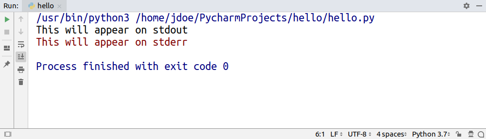
While both stdout and stderr are write-only, stdin is read-only. You can think of standard input as your keyboard, but just like with the other two, you can swap out stdin for a file to read data from.
In Python, you can access all standard streams through the built-in sys module:
>>> import sys
>>> sys.stdin
<_io.TextIOWrapper name='<stdin>' mode='r' encoding='UTF-8'>
>>> sys.stdin.fileno()
0
>>> sys.stdout
<_io.TextIOWrapper name='<stdout>' mode='w' encoding='UTF-8'>
>>> sys.stdout.fileno()
1
>>> sys.stderr
<_io.TextIOWrapper name='<stderr>' mode='w' encoding='UTF-8'>
>>> sys.stderr.fileno()
2
As you can see, these predefined values resemble file-like objects with mode and encoding attributes as well as .read() and .write() methods among many others.
By default, print() is bound to sys.stdout through its file argument, but you can change that. Use that keyword argument to indicate a file that was open in write or append mode, so that messages go straight to it:
with open('file.txt', mode='w') as file_object:
print('hello world', file=file_object)
This will make your code immune to stream redirection at the operating system level, which might or might not be desired.
For more information on working with files in Python, you can check out Reading and Writing Files in Python (Guide).
Note: Don’t try using print() for writing binary data as it’s only well suited for text.
Just call the binary file’s .write() directly:
with open('file.dat', 'wb') as file_object:
file_object.write(bytes(4))
file_object.write(b'\xff')
If you wanted to write raw bytes on the standard output, then this will fail too because sys.stdout is a character stream:
>>> import sys
>>> sys.stdout.write(bytes(4))
Traceback (most recent call last):
File "<stdin>", line 1, in <module>
TypeError: write() argument must be str, not bytes
You must dig deeper to get a handle of the underlying byte stream instead:
>>> import sys
>>> num_bytes_written = sys.stdout.buffer.write(b'\x41\x0a')
A
This prints an uppercase letter A and a newline character, which correspond to decimal values of 65 and 10 in ASCII. However, they’re encoded using hexadecimal notation in the bytes literal.
Note that print() has no control over character encoding. It’s the stream’s responsibility to encode received Unicode strings into bytes correctly. In most cases, you won’t set the encoding yourself, because the default UTF-8 is what you want. If you really need to, perhaps for legacy systems, you can use the encoding argument of open():
with open('file.txt', mode='w', encoding='iso-8859-1') as file_object:
print('über naïve café', file=file_object)
Instead of a real file existing somewhere in your file system, you can provide a fake one, which would reside in your computer’s memory. You’ll use this technique later for mocking print() in unit tests:
>>> import io
>>> fake_file = io.StringIO()
>>> print('hello world', file=fake_file)
>>> fake_file.getvalue()
'hello world\n'
If you got to this point, then you’re left with only one keyword argument in print(), which you’ll see in the next subsection. It’s probably the least used of them all. Nevertheless, there are times when it’s absolutely necessary.
There’s a special syntax in Python 2 for replacing the default sys.stdout with a custom file in the print statement:
with open('file.txt', mode='w') as file_object:
print >> file_object, 'hello world'
Because strings and bytes are represented with the same str type in Python 2, the print statement can handle binary data just fine:
with open('file.dat', mode='wb') as file_object:
print >> file_object, '\x41\x0a'
Although, there’s a problem with character encoding. The open() function in Python 2 lacks the encoding parameter, which would often result in the dreadful UnicodeEncodeError:
>>> with open('file.txt', mode='w') as file_object:
... unicode_text = u'\xfcber na\xefve caf\xe9'
... print >> file_object, unicode_text
...
Traceback (most recent call last):
File "<stdin>", line 3, in <module>
UnicodeEncodeError: 'ascii' codec can't encode character u'\xfc'...
Notice how non-Latin characters must be escaped in both Unicode and string literals to avoid a syntax error. Take a look at this example:
unicode_literal = u'\xfcber na\xefve caf\xe9'
string_literal = '\xc3\xbcber na\xc3\xafve caf\xc3\xa9'
Alternatively, you could specify source code encoding according to PEP 263 at the top of the file, but that wasn’t the best practice due to portability issues:
#!/usr/bin/env python2
# -*- coding: utf-8 -*-
unescaped_unicode_literal = u'über naïve café'
unescaped_string_literal = 'über naïve café'
Your best bet is to encode the Unicode string just before printing it. You can do this manually:
with open('file.txt', mode='w') as file_object:
unicode_text = u'\xfcber na\xefve caf\xe9'
encoded_text = unicode_text.encode('utf-8')
print >> file_object, encoded_text
However, a more convenient option is to use the built-in codecs module:
import codecs
with codecs.open('file.txt', 'w', encoding='utf-8') as file_object:
unicode_text = u'\xfcber na\xefve caf\xe9'
print >> file_object, unicode_text
It’ll take care of making appropriate conversions when you need to read or write files.
In the previous subsection, you learned that print() delegates printing to a file-like object such as sys.stdout. Some streams, however, buffer certain I/O operations to enhance performance, which can get in the way. Let’s take a look at an example.
Imagine you were writing a countdown timer, which should append the remaining time to the same line every second:
3...2...1...Go!
Your first attempt may look something like this:
import time
num_seconds = 3
for countdown in reversed(range(num_seconds + 1)):
if countdown > 0:
print(countdown, end='...')
time.sleep(1)
else:
print('Go!')
As long as the countdown variable is greater than zero, the code keeps appending text without a trailing newline and then goes to sleep for one second. Finally, when the countdown is finished, it prints Go! and terminates the line.
Unexpectedly, instead of counting down every second, the program idles wastefully for three seconds, and then suddenly prints the entire line at once:
That’s because the operating system buffers subsequent writes to the standard output in this case. You need to know that there are three kinds of streams with respect to buffering:
Unbuffered is self-explanatory, that is, no buffering is taking place, and all writes have immediate effect. A line-buffered stream waits before firing any I/O calls until a line break appears somewhere in the buffer, whereas a block-buffered one simply allows the buffer to fill up to a certain size regardless of its content. Standard output is both line-buffered and block-buffered, depending on which event comes first.
Buffering helps to reduce the number of expensive I/O calls. Think about sending messages over a high-latency network, for example. When you connect to a remote server to execute commands over the SSH protocol, each of your keystrokes may actually produce an individual data packet, which is orders of magnitude bigger than its payload. What an overhead! It would make sense to wait until at least a few characters are typed and then send them together. That’s where buffering steps in.
On the other hand, buffering can sometimes have undesired effects as you just saw with the countdown example. To fix it, you can simply tell print() to forcefully flush the stream without waiting for a newline character in the buffer using its flush flag:
print(countdown, end='...', flush=True)
That’s all. Your countdown should work as expected now, but don’t take my word for it. Go ahead and test it to see the difference.
Congratulations! At this point, you’ve seen examples of calling print() that cover all of its parameters. You know their purpose and when to use them. Understanding the signature is only the beginning, however. In the upcoming sections, you’ll see why.
There isn’t an easy way to flush the stream in Python 2, because the print statement doesn’t allow for it by itself. You need to get a handle of its lower-level layer, which is the standard output, and call it directly:
import time
import sys
num_seconds = 3
for countdown in reversed(range(num_seconds + 1)):
if countdown > 0:
sys.stdout.write('%s...' % countdown)
sys.stdout.flush()
time.sleep(1)
else:
print 'Go!'
Alternatively, you could disable buffering of the standard streams either by providing the -u flag to the Python interpreter or by setting up the PYTHONUNBUFFERED environment variable:
$ python2 -u countdown.py
$ PYTHONUNBUFFERED=1 python2 countdown.py
Note that print() was backported to Python 2 and made available through the __future__ module. Unfortunately, it doesn’t come with the flush parameter:
>>> from __future__ import print_function
>>> help(print)
Help on built-in function print in module __builtin__:
print(...)
print(value, ..., sep=' ', end='\n', file=sys.stdout)
What you’re seeing here is a docstring of the print() function. You can display docstrings of various objects in Python using the built-in help() function.
Up until now, you only dealt with built-in data types such as strings and numbers, but you’ll often want to print your own abstract data types. Let’s have a look at different ways of defining them.
For simple objects without any logic, whose purpose is to carry data, you’ll typically take advantage of namedtuple, which is available in the standard library. Named tuples have a neat textual representation out of the box:
>>> from collections import namedtuple
>>> Person = namedtuple('Person', 'name age')
>>> jdoe = Person('John Doe', 42)
>>> print(jdoe)
Person(name='John Doe', age=42)
That’s great as long as holding data is enough, but in order to add behaviors to the Person type, you’ll eventually need to define a class. Take a look at this example:
class Person:
def __init__(self, name, age):
self.name, self.age = name, age
If you now create an instance of the Person class and try to print it, you’ll get this bizarre output, which is quite different from the equivalent namedtuple:
>>> jdoe = Person('John Doe', 42)
>>> print(jdoe)
<__main__.Person object at 0x7fcac3fed1d0>
It’s the default representation of objects, which comprises their address in memory, the corresponding class name and a module in which they were defined. You’ll fix that in a bit, but just for the record, as a quick workaround you could combine namedtuple and a custom class through inheritance:
from collections import namedtuple
class Person(namedtuple('Person', 'name age')):
pass
Your Person class has just become a specialized kind of namedtuple with two attributes, which you can customize.
Note: In Python 3, the pass statement can be replaced with the ellipsis (...) literal to indicate a placeholder:
def delta(a, b, c):
...
This prevents the interpreter from raising IndentationError due to missing indented block of code.
That’s better than a plain namedtuple, because not only do you get printing right for free, but you can also add custom methods and properties to the class. However, it solves one problem while introducing another. Remember that tuples, including named tuples, are immutable in Python, so they can’t change their values once created.
It’s true that designing immutable data types is desirable, but in many cases, you’ll want them to allow for change, so you’re back with regular classes again.
Note: Following other languages and frameworks, Python 3.7 introduced data classes, which you can think of as mutable tuples. This way, you get the best of both worlds:
>>> from dataclasses import dataclass
>>> @dataclass
... class Person:
... name: str
... age: int
...
... def celebrate_birthday(self):
... self.age += 1
...
>>> jdoe = Person('John Doe', 42)
>>> jdoe.celebrate_birthday()
>>> print(jdoe)
Person(name='John Doe', age=43)
The syntax for variable annotations, which is required to specify class fields with their corresponding types, was defined in Python 3.6.
From earlier subsections, you already know that print() implicitly calls the built-in str() function to convert its positional arguments into strings. Indeed, calling str() manually against an instance of the regular Person class yields the same result as printing it:
>>> jdoe = Person('John Doe', 42)
>>> str(jdoe)
'<__main__.Person object at 0x7fcac3fed1d0>'
str(), in turn, looks for one of two magic methods within the class body, which you typically implement. If it doesn’t find one, then it falls back to the ugly default representation. Those magic methods are, in order of search:
def __str__(self)def __repr__(self)The first one is recommended to return a short, human-readable text, which includes information from the most relevant attributes. After all, you don’t want to expose sensitive data, such as user passwords, when printing objects.
However, the other one should provide complete information about an object, to allow for restoring its state from a string. Ideally, it should return valid Python code, so that you can pass it directly to eval():
>>> repr(jdoe)
"Person(name='John Doe', age=42)"
>>> type(eval(repr(jdoe)))
<class '__main__.Person'>
Notice the use of another built-in function, repr(), which always tries to call .__repr__() in an object, but falls back to the default representation if it doesn’t find that method.
Note: Even though print() itself uses str() for type casting, some compound data types delegate that call to repr() on their members. This happens to lists and tuples, for example.
Consider this class with both magic methods, which return alternative string representations of the same object:
class User:
def __init__(self, login, password):
self.login = login
self.password = password
def __str__(self):
return self.login
def __repr__(self):
return f"User('{self.login}', '{self.password}')"
If you print a single object of the User class, then you won’t see the password, because print(user) will call str(user), which eventually will invoke user.__str__():
>>> user = User('jdoe', 's3cret')
>>> print(user)
jdoe
However, if you put the same user variable inside a list by wrapping it in square brackets, then the password will become clearly visible:
>>> print([user])
[User('jdoe', 's3cret')]
That’s because sequences, such as lists and tuples, implement their .__str__() method so that all of their elements are first converted with repr().
Python gives you a lot of freedom when it comes to defining your own data types if none of the built-in ones meet your needs. Some of them, such as named tuples and data classes, offer string representations that look good without requiring any work on your part. Still, for the most flexibility, you’ll have to define a class and override its magic methods described above.
The semantics of .__str__() and .__repr__() didn’t change since Python 2, but you must remember that strings were nothing more than glorified byte arrays back then. To convert your objects into proper Unicode, which was a separate data type, you’d have to provide yet another magic method: .__unicode__().
Here’s an example of the same User class in Python 2:
class User(object):
def __init__(self, login, password):
self.login = login
self.password = password
def __unicode__(self):
return self.login
def __str__(self):
return unicode(self).encode('utf-8')
def __repr__(self):
user = u"User('%s', '%s')" % (self.login, self.password)
return user.encode('unicode_escape')
As you can see, this implementation delegates some work to avoid duplication by calling the built-in unicode() function on itself.
Both .__str__() and .__repr__() methods must return strings, so they encode Unicode characters into specific byte representations called character sets. UTF-8 is the most widespread and safest encoding, while unicode_escape is a special constant to express funky characters, such as é, as escape sequences in plain ASCII, such as \xe9.
The print statement is looking for the magic .__str__() method in the class, so the chosen charset must correspond to the one used by the terminal. For example, default encoding in DOS and Windows is CP 852 rather than UTF-8, so running this can result in a UnicodeEncodeError or even garbled output:
>>> user = User(u'\u043d\u0438\u043a\u0438\u0442\u0430', u's3cret')
>>> print user
đŻđŞđ║đŞĐéđ░
However, if you ran the same code on a system with UTF-8 encoding, then you’d get the proper spelling of a popular Russian name:
>>> user = User(u'\u043d\u0438\u043a\u0438\u0442\u0430', u's3cret')
>>> print user
никита
It’s recommended to convert strings to Unicode as early as possible, for example, when you’re reading data from a file, and use it consistently everywhere in your code. At the same time, you should encode Unicode back to the chosen character set right before presenting it to the user.
It seems as if you have more control over string representation of objects in Python 2 because there’s no magic .__unicode__() method in Python 3 anymore. You may be asking yourself if it’s possible to convert an object to its byte string representation rather than a Unicode string in Python 3. It’s possible, with a special .__bytes__() method that does just that:
>>> class User(object):
... def __init__(self, login, password):
... self.login = login
... self.password = password
...
... def __bytes__(self): # Python 3
... return self.login.encode('utf-8')
...
>>> user = User(u'\u043d\u0438\u043a\u0438\u0442\u0430', u's3cret')
>>> bytes(user)
b'\xd0\xbd\xd0\xb8\xd0\xba\xd0\xb8\xd1\x82\xd0\xb0'
Using the built-in bytes() function on an instance delegates the call to its __bytes__() method defined in the corresponding class.
You know how to use print() quite well at this point, but knowing what it is will allow you to use it even more effectively and consciously. After reading this section, you’ll understand how printing in Python has improved over the years.
You’ve seen that print() is a function in Python 3. More specifically, it’s a built-in function, which means that you don’t need to import it from anywhere:
>>> print
<built-in function print>
It’s always available in the global namespace so that you can call it directly, but you can also access it through a module from the standard library:
>>> import builtins
>>> builtins.print
<built-in function print>
This way, you can avoid name collisions with custom functions. Let’s say you wanted to redefine print() so that it doesn’t append a trailing newline. At the same time, you wanted to rename the original function to something like println():
>>> import builtins
>>> println = builtins.print
>>> def print(*args, **kwargs):
... builtins.print(*args, **kwargs, end='')
...
>>> println('hello')
hello
>>> print('hello\n')
hello
Now you have two separate printing functions just like in the Java programming language. You’ll define custom print() functions in the mocking section later as well. Also, note that you wouldn’t be able to overwrite print() in the first place if it wasn’t a function.
On the other hand, print() isn’t a function in the mathematical sense, because it doesn’t return any meaningful value other than the implicit None:
>>> value = print('hello world')
hello world
>>> print(value)
None
Such functions are, in fact, procedures or subroutines that you call to achieve some kind of side-effect, which ultimately is a change of a global state. In the case of print(), that side-effect is showing a message on the standard output or writing to a file.
Because print() is a function, it has a well-defined signature with known attributes. You can quickly find its documentation using the editor of your choice, without having to remember some weird syntax for performing a certain task.
Besides, functions are easier to extend. Adding a new feature to a function is as easy as adding another keyword argument, whereas changing the language to support that new feature is much more cumbersome. Think of stream redirection or buffer flushing, for example.
Another benefit of print() being a function is composability. Functions are so-called first-class objects or first-class citizens in Python, which is a fancy way of saying they’re values just like strings or numbers. This way, you can assign a function to a variable, pass it to another function, or even return one from another. print() isn’t different in this regard. For instance, you can take advantage of it for dependency injection:
def download(url, log=print):
log(f'Downloading {url}')
# ...
def custom_print(*args):
pass # Do not print anything
download('/js/app.js', log=custom_print)
Here, the log parameter lets you inject a callback function, which defaults to print() but can be any callable. In this example, printing is completely disabled by substituting print() with a dummy function that does nothing.
Note: A dependency is any piece of code required by another bit of code.
Dependency injection is a technique used in code design to make it more testable, reusable, and open for extension. You can achieve it by referring to dependencies indirectly through abstract interfaces and by providing them in a push rather than pull fashion.
There’s a funny explanation of dependency injection circulating on the Internet:
Dependency injection for five-year-olds
When you go and get things out of the refrigerator for yourself, you can cause problems. You might leave the door open, you might get something Mommy or Daddy doesn’t want you to have. You might even be looking for something we don’t even have or which has expired.
What you should be doing is stating a need, “I need something to drink with lunch,” and then we will make sure you have something when you sit down to eat.
— John Munsch, 28 October 2009. (Source)
Composition allows you to combine a few functions into a new one of the same kind. Let’s see this in action by specifying a custom error() function that prints to the standard error stream and prefixes all messages with a given log level:
>>> from functools import partial
>>> import sys
>>> redirect = lambda function, stream: partial(function, file=stream)
>>> prefix = lambda function, prefix: partial(function, prefix)
>>> error = prefix(redirect(print, sys.stderr), '[ERROR]')
>>> error('Something went wrong')
[ERROR] Something went wrong
This custom function uses partial functions to achieve the desired effect. It’s an advanced concept borrowed from the functional programming paradigm, so you don’t need to go too deep into that topic for now. However, if you’re interested in this topic, I recommend taking a look at the functools module.
Unlike statements, functions are values. That means you can mix them with expressions, in particular, lambda expressions. Instead of defining a full-blown function to replace print() with, you can make an anonymous lambda expression that calls it:
>>> download('/js/app.js', lambda msg: print('[INFO]', msg))
[INFO] Downloading /js/app.js
However, because a lambda expression is defined in place, there’s no way of referring to it elsewhere in the code.
Note: In Python, you can’t put statements, such as assignments, conditional statements, loops, and so on, in an anonymous lambda function. It has to be a single expression!
Another kind of expression is a ternary conditional expression:
>>> user = 'jdoe'
>>> print('Hi!') if user is None else print(f'Hi, {user}.')
Hi, jdoe.
Python has both conditional statements and conditional expressions. The latter is evaluated to a single value that can be assigned to a variable or passed to a function. In the example above, you’re interested in the side-effect rather than the value, which evaluates to None, so you simply ignore it.
As you can see, functions allow for an elegant and extensible solution, which is consistent with the rest of the language. In the next subsection, you’ll discover how not having print() as a function caused a lot of headaches.
A statement is an instruction that may evoke a side-effect when executed but never evaluates to a value. In other words, you wouldn’t be able to print a statement or assign it to a variable like this:
result = print 'hello world'
That’s a syntax error in Python 2.
Here are a few more examples of statements in Python:
=ifwhileassertNote: Python 3.8 brings a controversial walrus operator (:=), which is an assignment expression. With it, you can evaluate an expression and assign the result to a variable at the same time, even within another expression!
Take a look at this example, which calls an expensive function once and then reuses the result for further computation:
# Python 3.8+
values = [y := f(x), y**2, y**3]
This is useful for simplifying the code without losing its efficiency. Typically, performant code tends to be more verbose:
y = f(x)
values = [y, y**2, y**3]
The controversy behind this new piece of syntax caused a lot of argument. An abundance of negative comments and heated debates eventually led Guido van Rossum to step down from the Benevolent Dictator For Life or BDFL position.
Statements are usually comprised of reserved keywords such as if, for, or print that have fixed meaning in the language. You can’t use them to name your variables or other symbols. That’s why redefining or mocking the print statement isn’t possible in Python 2. You’re stuck with what you get.
Furthermore, you can’t print from anonymous functions, because statements aren’t accepted in lambda expressions:
>>> lambda: print 'hello world'
File "<stdin>", line 1
lambda: print 'hello world'
^
SyntaxError: invalid syntax
The syntax of the print statement is ambiguous. Sometimes you can add parentheses around the message, and they’re completely optional:
>>> print 'Please wait...'
Please wait...
>>> print('Please wait...')
Please wait...
At other times they change how the message is printed:
>>> print 'My name is', 'John'
My name is John
>>> print('My name is', 'John')
('My name is', 'John')
String concatenation can raise a TypeError due to incompatible types, which you have to handle manually, for example:
>>> values = ['jdoe', 'is', 42, 'years old']
>>> print ' '.join(map(str, values))
jdoe is 42 years old
Compare this with similar code in Python 3, which leverages sequence unpacking:
>>> values = ['jdoe', 'is', 42, 'years old']
>>> print(*values) # Python 3
jdoe is 42 years old
There aren’t any keyword arguments for common tasks such as flushing the buffer or stream redirection. You need to remember the quirky syntax instead. Even the built-in help() function isn’t that helpful with regards to the print statement:
>>> help(print)
File "<stdin>", line 1
help(print)
^
SyntaxError: invalid syntax
Trailing newline removal doesn’t work quite right, because it adds an unwanted space. You can’t compose multiple print statements together, and, on top of that, you have to be extra diligent about character encoding.
The list of problems goes on and on. If you’re curious, you can jump back to the previous section and look for more detailed explanations of the syntax in Python 2.
However, you can mitigate some of those problems with a much simpler approach. It turns out the print() function was backported to ease the migration to Python 3. You can import it from a special __future__ module, which exposes a selection of language features released in later Python versions.
Note: You may import future functions as well as baked-in language constructs such as the with statement.
To find out exactly what features are available to you, inspect the module:
>>> import __future__
>>> __future__.all_feature_names
['nested_scopes',
'generators',
'division',
'absolute_import',
'with_statement',
'print_function',
'unicode_literals']
You could also call dir(__future__), but that would show a lot of uninteresting internal details of the module.
To enable the print() function in Python 2, you need to add this import statement at the beginning of your source code:
from __future__ import print_function
From now on the print statement is no longer available, but you have the print() function at your disposal. Note that it isn’t the same function like the one in Python 3, because it’s missing the flush keyword argument, but the rest of the arguments are the same.
Other than that, it doesn’t spare you from managing character encodings properly.
Here’s an example of calling the print() function in Python 2:
>>> from __future__ import print_function
>>> import sys
>>> print('I am a function in Python', sys.version_info.major)
I am a function in Python 2
You now have an idea of how printing in Python evolved and, most importantly, understand why these backward-incompatible changes were necessary. Knowing this will surely help you become a better Python programmer.
If you thought that printing was only about lighting pixels up on the screen, then technically you’d be right. However, there are ways to make it look cool. In this section, you’ll find out how to format complex data structures, add colors and other decorations, build interfaces, use animation, and even play sounds with text!
Computer languages allow you to represent data as well as executable code in a structured way. Unlike Python, however, most languages give you a lot of freedom in using whitespace and formatting. This can be useful, for example in compression, but it sometimes leads to less readable code.
Pretty-printing is about making a piece of data or code look more appealing to the human eye so that it can be understood more easily. This is done by indenting certain lines, inserting newlines, reordering elements, and so forth.
Python comes with the pprint module in its standard library, which will help you in pretty-printing large data structures that don’t fit on a single line. Because it prints in a more human-friendly way, many popular REPL tools, including JupyterLab and IPython, use it by default in place of the regular print() function.
Note: To toggle pretty printing in IPython, issue the following command:
In [1]: %pprint
Pretty printing has been turned OFF
In [2]: %pprint
Pretty printing has been turned ON
This is an example of Magic in IPython. There are a lot of built-in commands that start with a percent sign (%), but you can find more on PyPI, or even create your own.
If you don’t care about not having access to the original print() function, then you can replace it with pprint() in your code using import renaming:
>>> from pprint import pprint as print
>>> print
<function pprint at 0x7f7a775a3510>
Personally, I like to have both functions at my fingertips, so I’d rather use something like pp as a short alias:
from pprint import pprint as pp
At first glance, there’s hardly any difference between the two functions, and in some cases there’s virtually none:
>>> print(42)
42
>>> pp(42)
42
>>> print('hello')
hello
>>> pp('hello')
'hello' # Did you spot the difference?
That’s because pprint() calls repr() instead of the usual str() for type casting, so that you may evaluate its output as Python code if you want to. The differences become apparent as you start feeding it more complex data structures:
>>> data = {'powers': [x**10 for x in range(10)]}
>>> pp(data)
{'powers': [0,
1,
1024,
59049,
1048576,
9765625,
60466176,
282475249,
1073741824,
3486784401]}
The function applies reasonable formatting to improve readability, but you can customize it even further with a couple of parameters. For example, you may limit a deeply nested hierarchy by showing an ellipsis below a given level:
>>> cities = {'USA': {'Texas': {'Dallas': ['Irving']}}}
>>> pp(cities, depth=3)
{'USA': {'Texas': {'Dallas': [...]}}}
The ordinary print() also uses ellipses but for displaying recursive data structures, which form a cycle, to avoid stack overflow error:
>>> items = [1, 2, 3]
>>> items.append(items)
>>> print(items)
[1, 2, 3, [...]]
However, pprint() is more explicit about it by including the unique identity of a self-referencing object:
>>> pp(items)
[1, 2, 3, <Recursion on list with id=140635757287688>]
>>> id(items)
140635757287688
The last element in the list is the same object as the entire list.
Note: Recursive or very large data sets can be dealt with using the reprlib module as well:
>>> import reprlib
>>> reprlib.repr([x**10 for x in range(10)])
'[0, 1, 1024, 59049, 1048576, 9765625, ...]'
This module supports most of the built-in types and is used by the Python debugger.
pprint() automatically sorts dictionary keys for you before printing, which allows for consistent comparison. When you’re comparing strings, you often don’t care about a particular order of serialized attributes. Anyways, it’s always best to compare actual dictionaries before serialization.
Dictionaries often represent JSON data, which is widely used on the Internet. To correctly serialize a dictionary into a valid JSON-formatted string, you can take advantage of the json module. It too has pretty-printing capabilities:
>>> import json
>>> data = {'username': 'jdoe', 'password': 's3cret'}
>>> ugly = json.dumps(data)
>>> pretty = json.dumps(data, indent=4, sort_keys=True)
>>> print(ugly)
{"username": "jdoe", "password": "s3cret"}
>>> print(pretty)
{
"password": "s3cret",
"username": "jdoe"
}
Notice, however, that you need to handle printing yourself, because it’s not something you’d typically want to do. Similarly, the pprint module has an additional pformat() function that returns a string, in case you had to do something other than printing it.
Surprisingly, the signature of pprint() is nothing like the print() function’s one. You can’t even pass more than one positional argument, which shows how much it focuses on printing data structures.
As personal computers got more sophisticated, they had better graphics and could display more colors. However, different vendors had their own idea about the API design for controlling it. That changed a few decades ago when people at the American National Standards Institute decided to unify it by defining ANSI escape codes.
Most of today’s terminal emulators support this standard to some degree. Until recently, the Windows operating system was a notable exception. Therefore, if you want the best portability, use the colorama library in Python. It translates ANSI codes to their appropriate counterparts in Windows while keeping them intact in other operating systems.
To check if your terminal understands a subset of the ANSI escape sequences, for example, related to colors, you can try using the following command:
$ tput colors
My default terminal on Linux says it can display 256 distinct colors, while xterm gives me only 8. The command would return a negative number if colors were unsupported.
ANSI escape sequences are like a markup language for the terminal. In HTML you work with tags, such as <b> or <i>, to change how elements look in the document. These tags are mixed with your content, but they’re not visible themselves. Similarly, escape codes won’t show up in the terminal as long as it recognizes them. Otherwise, they’ll appear in the literal form as if you were viewing the source of a website.
As its name implies, a sequence must begin with the non-printable Esc character, whose ASCII value is 27, sometimes denoted as 0x1b in hexadecimal or 033 in octal. You may use Python number literals to quickly verify it’s indeed the same number:
>>> 27 == 0x1b == 0o33
True
Additionally, you can obtain it with the \e escape sequence in the shell:
$ echo -e "\e"
The most common ANSI escape sequences take the following form:
| Element | Description | Example |
|---|---|---|
| Esc | non-printable escape character | \033 |
[ |
opening square bracket | [ |
| numeric code | one or more numbers separated with ; |
0 |
| character code | uppercase or lowercase letter | m |
The numeric code can be one or more numbers separated with a semicolon, while the character code is just one letter. Their specific meaning is defined by the ANSI standard. For example, to reset all formatting, you would type one of the following commands, which use the code zero and the letter m:
$ echo -e "\e[0m"
$ echo -e "\x1b[0m"
$ echo -e "\033[0m"
At the other end of the spectrum, you have compound code values. To set foreground and background with RGB channels, given that your terminal supports 24-bit depth, you could provide multiple numbers:
$ echo -e "\e[38;2;0;0;0m\e[48;2;255;255;255mBlack on white\e[0m"
It’s not just text color that you can set with the ANSI escape codes. You can, for example, clear and scroll the terminal window, change its background, move the cursor around, make the text blink or decorate it with an underline.
In Python, you’d probably write a helper function to allow for wrapping arbitrary codes into a sequence:
>>> def esc(code):
... return f'\033[{code}m'
...
>>> print(esc('31;1;4') + 'really' + esc(0) + ' important')
This would make the word really appear in red, bold, and underlined font:
However, there are higher-level abstractions over ANSI escape codes, such as the mentioned colorama library, as well as tools for building user interfaces in the console.
While playing with ANSI escape codes is undeniably a ton of fun, in the real world you’d rather have more abstract building blocks to put together a user interface. There are a few libraries that provide such a high level of control over the terminal, but curses seems to be the most popular choice.
Note: To use the curses library in Windows, you need to install a third-party package:
C:\> pip install windows-curses
That’s because curses isn’t available in the standard library of the Python distribution for Windows.
Primarily, it allows you to think in terms of independent graphical widgets instead of a blob of text. Besides, you get a lot of freedom in expressing your inner artist, because it’s really like painting a blank canvas. The library hides the complexities of having to deal with different terminals. Other than that, it has great support for keyboard events, which might be useful for writing video games.
How about making a retro snake game? Let’s create a Python snake simulator:
First, you need to import the curses module. Since it modifies the state of a running terminal, it’s important to handle errors and gracefully restore the previous state. You can do this manually, but the library comes with a convenient wrapper for your main function:
import curses
def main(screen):
pass
if __name__ == '__main__':
curses.wrapper(main)
Note, the function must accept a reference to the screen object, also known as stdscr, that you’ll use later for additional setup.
If you run this program now, you won’t see any effects, because it terminates immediately. However, you can add a small delay to have a sneak peek:
import time, curses
def main(screen):
time.sleep(1)
if __name__ == '__main__':
curses.wrapper(main)
This time the screen went completely blank for a second, but the cursor was still blinking. To hide it, just call one of the configuration functions defined in the module:
import time, curses
def main(screen):
curses.curs_set(0) # Hide the cursor
time.sleep(1)
if __name__ == '__main__':
curses.wrapper(main)
Let’s define the snake as a list of points in screen coordinates:
snake = [(0, i) for i in reversed(range(20))]
The head of the snake is always the first element in the list, whereas the tail is the last one. The initial shape of the snake is horizontal, starting from the top-left corner of the screen and facing to the right. While its y-coordinate stays at zero, its x-coordinate decreases from head to tail.
To draw the snake, you’ll start with the head and then follow with the remaining segments. Each segment carries (y, x) coordinates, so you can unpack them:
# Draw the snake
screen.addstr(*snake[0], '@')
for segment in snake[1:]:
screen.addstr(*segment, '*')
Again, if you run this code now, it won’t display anything, because you must explicitly refresh the screen afterward:
import time, curses
def main(screen):
curses.curs_set(0) # Hide the cursor
snake = [(0, i) for i in reversed(range(20))]
# Draw the snake
screen.addstr(*snake[0], '@')
for segment in snake[1:]:
screen.addstr(*segment, '*')
screen.refresh()
time.sleep(1)
if __name__ == '__main__':
curses.wrapper(main)
You want to move the snake in one of four directions, which can be defined as vectors. Eventually, the direction will change in response to an arrow keystroke, so you may hook it up to the library’s key codes:
directions = {
curses.KEY_UP: (-1, 0),
curses.KEY_DOWN: (1, 0),
curses.KEY_LEFT: (0, -1),
curses.KEY_RIGHT: (0, 1),
}
direction = directions[curses.KEY_RIGHT]
How does a snake move? It turns out that only its head really moves to a new location, while all other segments shift towards it. In each step, almost all segments remain the same, except for the head and the tail. Assuming the snake isn’t growing, you can remove the tail and insert a new head at the beginning of the list:
# Move the snake
snake.pop()
snake.insert(0, tuple(map(sum, zip(snake[0], direction))))
To get the new coordinates of the head, you need to add the direction vector to it. However, adding tuples in Python results in a bigger tuple instead of the algebraic sum of the corresponding vector components. One way to fix this is by using the built-in zip(), sum(), and map() functions.
The direction will change on a keystroke, so you need to call .getch() to obtain the pressed key code. However, if the pressed key doesn’t correspond to the arrow keys defined earlier as dictionary keys, the direction won’t change:
# Change direction on arrow keystroke
direction = directions.get(screen.getch(), direction)
By default, however, .getch() is a blocking call that would prevent the snake from moving unless there was a keystroke. Therefore, you need to make the call non-blocking by adding yet another configuration:
def main(screen):
curses.curs_set(0) # Hide the cursor
screen.nodelay(True) # Don't block I/O calls
You’re almost done, but there’s just one last thing left. If you now loop this code, the snake will appear to be growing instead of moving. That’s because you have to erase the screen explicitly before each iteration.
Finally, this is all you need to play the snake game in Python:
import time, curses
def main(screen):
curses.curs_set(0) # Hide the cursor
screen.nodelay(True) # Don't block I/O calls
directions = {
curses.KEY_UP: (-1, 0),
curses.KEY_DOWN: (1, 0),
curses.KEY_LEFT: (0, -1),
curses.KEY_RIGHT: (0, 1),
}
direction = directions[curses.KEY_RIGHT]
snake = [(0, i) for i in reversed(range(20))]
while True:
screen.erase()
# Draw the snake
screen.addstr(*snake[0], '@')
for segment in snake[1:]:
screen.addstr(*segment, '*')
# Move the snake
snake.pop()
snake.insert(0, tuple(map(sum, zip(snake[0], direction))))
# Change direction on arrow keystroke
direction = directions.get(screen.getch(), direction)
screen.refresh()
time.sleep(0.1)
if __name__ == '__main__':
curses.wrapper(main)
This is merely scratching the surface of the possibilities that the curses module opens up. You may use it for game development like this or more business-oriented applications.
Not only can animations make the user interface more appealing to the eye, but they also improve the overall user experience. When you provide early feedback to the user, for example, they’ll know if your program’s still working or if it’s time to kill it.
To animate text in the terminal, you have to be able to freely move the cursor around. You can do this with one of the tools mentioned previously, that is ANSI escape codes or the curses library. However, I’d like to show you an even simpler way.
If the animation can be constrained to a single line of text, then you might be interested in two special escape character sequences:
\r\bThe first one moves the cursor to the beginning of the line, whereas the second one moves it only one character to the left. They both work in a non-destructive way without overwriting text that’s already been written.
Let’s take a look at a few examples.
You’ll often want to display some kind of a spinning wheel to indicate a work in progress without knowing exactly how much time’s left to finish:
Many command line tools use this trick while downloading data over the network. You can make a really simple stop motion animation from a sequence of characters that will cycle in a round-robin fashion:
from itertools import cycle
from time import sleep
for frame in cycle(r'-\|/-\|/'):
print('\r', frame, sep='', end='', flush=True)
sleep(0.2)
The loop gets the next character to print, then moves the cursor to the beginning of the line, and overwrites whatever there was before without adding a newline. You don’t want extra space between positional arguments, so separator argument must be blank. Also, notice the use of Python’s raw strings due to backslash characters present in the literal.
When you know the remaining time or task completion percentage, then you’re able to show an animated progress bar:
First, you need to calculate how many hashtags to display and how many blank spaces to insert. Next, you erase the line and build the bar from scratch:
from time import sleep
def progress(percent=0, width=30):
left = width * percent // 100
right = width - left
print('\r[', '#' * left, ' ' * right, ']',
f' {percent:.0f}%',
sep='', end='', flush=True)
for i in range(101):
progress(i)
sleep(0.1)
As before, each request for update repaints the entire line.
Note: There’s a feature-rich progressbar2 library, along with a few other similar tools, that can show progress in a much more comprehensive way.
If you’re old enough to remember computers with a PC speaker, then you must also remember their distinctive beep sound, often used to indicate hardware problems. They could barely make any more noises than that, yet video games seemed so much better with it.
Today you can still take advantage of this small loudspeaker, but chances are your laptop didn’t come with one. In such a case, you can enable terminal bell emulation in your shell, so that a system warning sound is played instead.
Go ahead and type this command to see if your terminal can play a sound:
$ echo -e "\a"
This would normally print text, but the -e flag enables the interpretation of backslash escapes. As you can see, there’s a dedicated escape sequence \a, which stands for “alert”, that outputs a special bell character. Some terminals make a sound whenever they see it.
Similarly, you can print this character in Python. Perhaps in a loop to form some kind of melody. While it’s only a single note, you can still vary the length of pauses between consecutive instances. That seems like a perfect toy for Morse code playback!
The rules are the following:
According to those rules, you could be “printing” an SOS signal indefinitely in the following way:
while True:
dot()
symbol_space()
dot()
symbol_space()
dot()
letter_space()
dash()
symbol_space()
dash()
symbol_space()
dash()
letter_space()
dot()
symbol_space()
dot()
symbol_space()
dot()
word_space()
In Python, you can implement it in merely ten lines of code:
from time import sleep
speed = 0.1
def signal(duration, symbol):
sleep(duration)
print(symbol, end='', flush=True)
dot = lambda: signal(speed, '·\a')
dash = lambda: signal(3*speed, '−\a')
symbol_space = lambda: signal(speed, '')
letter_space = lambda: signal(3*speed, '')
word_space = lambda: signal(7*speed, ' ')
Maybe you could even take it one step further and make a command line tool for translating text into Morse code? Either way, I hope you’re having fun with this!
Nowadays, it’s expected that you ship code that meets high quality standards. If you aspire to become a professional, you must learn how to test your code.
Software testing is especially important in dynamically typed languages, such as Python, which don’t have a compiler to warn you about obvious mistakes. Defects can make their way to the production environment and remain dormant for a long time, until that one day when a branch of code finally gets executed.
Sure, you have linters, type checkers, and other tools for static code analysis to assist you. But they won’t tell you whether your program does what it’s supposed to do on the business level.
So, should you be testing print()? No. After all, it’s a built-in function that must have already gone through a comprehensive suite of tests. What you want to test, though, is whether your code is calling print() at the right time with the expected parameters. That’s known as a behavior.
You can test behaviors by mocking real objects or functions. In this case, you want to mock print() to record and verify its invocations.
Note: You might have heard the terms: dummy, fake, stub, spy, or mock used interchangeably. Some people make a distinction between them, while others don’t.
Martin Fowler explains their differences in a short glossary and collectively calls them test doubles.
Mocking in Python can be done twofold. First, you can take the traditional path of statically-typed languages by employing dependency injection. This may sometimes require you to change the code under test, which isn’t always possible if the code is defined in an external library:
def download(url, log=print):
log(f'Downloading {url}')
# ...
This is the same example I used in an earlier section to talk about function composition. It basically allows for substituting print() with a custom function of the same interface. To check if it prints the right message, you have to intercept it by injecting a mocked function:
>>> def mock_print(message):
... mock_print.last_message = message
...
>>> download('resource', mock_print)
>>> assert 'Downloading resource' == mock_print.last_message
Calling this mock makes it save the last message in an attribute, which you can inspect later, for example in an assert statement.
In a slightly alternative solution, instead of replacing the entire print() function with a custom wrapper, you could redirect the standard output to an in-memory file-like stream of characters:
>>> def download(url, stream=None):
... print(f'Downloading {url}', file=stream)
... # ...
...
>>> import io
>>> memory_buffer = io.StringIO()
>>> download('app.js', memory_buffer)
>>> download('style.css', memory_buffer)
>>> memory_buffer.getvalue()
'Downloading app.js\nDownloading style.css\n'
This time the function explicitly calls print(), but it exposes its file parameter to the outside world.
However, a more Pythonic way of mocking objects takes advantage of the built-in mock module, which uses a technique called monkey patching. This derogatory name stems from it being a “dirty hack” that you can easily shoot yourself in the foot with. It’s less elegant than dependency injection but definitely quick and convenient.
Note: The mock module got absorbed by the standard library in Python 3, but before that, it was a third-party package. You had to install it separately:
$ pip2 install mock
Other than that, you referred to it as mock, whereas in Python 3 it’s part of the unit testing module, so you must import from unittest.mock.
What monkey patching does is alter implementation dynamically at runtime. Such a change is visible globally, so it may have unwanted consequences. In practice, however, patching only affects the code for the duration of test execution.
To mock print() in a test case, you’ll typically use the @patch decorator and specify a target for patching by referring to it with a fully qualified name, that is including the module name:
from unittest.mock import patch
@patch('builtins.print')
def test_print(mock_print):
print('not a real print')
mock_print.assert_called_with('not a real print')
This will automatically create the mock for you and inject it to the test function. However, you need to declare that your test function accepts a mock now. The underlying mock object has lots of useful methods and attributes for verifying behavior.
Did you notice anything peculiar about that code snippet?
Despite injecting a mock to the function, you’re not calling it directly, although you could. That injected mock is only used to make assertions afterward and maybe to prepare the context before running the test.
In real life, mocking helps to isolate the code under test by removing dependencies such as a database connection. You rarely call mocks in a test, because that doesn’t make much sense. Rather, it’s other pieces of code that call your mock indirectly without knowing it.
Here’s what that means:
from unittest.mock import patch
def greet(name):
print(f'Hello, {name}!')
@patch('builtins.print')
def test_greet(mock_print):
greet('John')
mock_print.assert_called_with('Hello, John!')
The code under test is a function that prints a greeting. Even though it’s a fairly simple function, you can’t test it easily because it doesn’t return a value. It has a side-effect.
To eliminate that side-effect, you need to mock the dependency out. Patching lets you avoid making changes to the original function, which can remain agnostic about print(). It thinks it’s calling print(), but in reality, it’s calling a mock you’re in total control of.
There are many reasons for testing software. One of them is looking for bugs. When you write tests, you often want to get rid of the print() function, for example, by mocking it away. Paradoxically, however, that same function can help you find bugs during a related process of debugging you’ll read about in the next section.
You can’t monkey patch the print statement in Python 2, nor can you inject it as a dependency. However, you have a few other options:
sys module.print() from the __future__ module.Let’s examine them one by one.
Stream redirection is almost identical to the example you saw earlier:
>>> def download(url, stream=None):
... print >> stream, 'Downloading %s' % url
... # ...
...
>>> from StringIO import StringIO
>>> memory_buffer = StringIO()
>>> download('app.js', memory_buffer)
>>> download('style.css', memory_buffer)
>>> memory_buffer.getvalue()
'Downloading app.js\nDownloading style.css\n'
There are only two differences. First, the syntax for stream redirection uses chevron (>>) instead of the file argument. The other difference is where StringIO is defined. You can import it from a similarly named StringIO module, or cStringIO for a faster implementation.
Patching the standard output from the sys module is exactly what it sounds like, but you need to be aware of a few gotchas:
from mock import patch, call
def greet(name):
print 'Hello, %s!' % name
@patch('sys.stdout')
def test_greet(mock_stdout):
greet('John')
mock_stdout.write.assert_has_calls([
call('Hello, John!'),
call('\n')
])
First of all, remember to install the mock module as it wasn’t available in the standard library in Python 2.
Secondly, the print statement calls the underlying .write() method on the mocked object instead of calling the object itself. That’s why you’ll run assertions against mock_stdout.write.
Finally, a single print statement doesn’t always correspond to a single call to sys.stdout.write(). In fact, you’ll see the newline character written separately.
The last option you have is importing print() from future and patching it:
from __future__ import print_function
from mock import patch
def greet(name):
print('Hello, %s!' % name)
@patch('__builtin__.print')
def test_greet(mock_print):
greet('John')
mock_print.assert_called_with('Hello, John!')
Again, it’s nearly identical to Python 3, but the print() function is defined in the __builtin__ module rather than builtins.
In this section, you’ll take a look at the available tools for debugging in Python, starting from a humble print() function, through the logging module, to a fully fledged debugger. After reading it, you’ll be able to make an educated decision about which of them is the most suitable in a given situation.
Note: Debugging is the process of looking for the root causes of bugs or defects in software after they’ve been discovered, as well as taking steps to fix them.
The term bug has an amusing story about the origin of its name.
Also known as print debugging or caveman debugging, it’s the most basic form of debugging. While a little bit old-fashioned, it’s still powerful and has its uses.
The idea is to follow the path of program execution until it stops abruptly, or gives incorrect results, to identify the exact instruction with a problem. You do that by inserting print statements with words that stand out in carefully chosen places.
Take a look at this example, which manifests a rounding error:
>>> def average(numbers):
... print('debug1:', numbers)
... if len(numbers) > 0:
... print('debug2:', sum(numbers))
... return sum(numbers) / len(numbers)
...
>>> 0.1 == average(3*[0.1])
debug1: [0.1, 0.1, 0.1]
debug2: 0.30000000000000004
False
As you can see, the function doesn’t return the expected value of 0.1, but now you know it’s because the sum is a little off. Tracing the state of variables at different steps of the algorithm can give you a hint where the issue is.
In this case, the problem lies in how floating point numbers are represented in computer memory. Remember that numbers are stored in binary form. Decimal value of 0.1 turns out to have an infinite binary representation, which gets rounded.
For more information on rounding numbers in Python, you can check out How to Round Numbers in Python.
This method is simple and intuitive and will work in pretty much every programming language out there. Not to mention, it’s a great exercise in the learning process.
On the other hand, once you master more advanced techniques, it’s hard to go back, because they allow you to find bugs much quicker. Tracing is a laborious manual process, which can let even more errors slip through. The build and deploy cycle takes time. Afterward, you need to remember to meticulously remove all the print() calls you made without accidentally touching the genuine ones.
Besides, it requires you to make changes in the code, which isn’t always possible. Maybe you’re debugging an application running in a remote web server or want to diagnose a problem in a post-mortem fashion. Sometimes you simply don’t have access to the standard output.
That’s precisely where logging shines.
Let’s pretend for a minute that you’re running an e-commerce website. One day, an angry customer makes a phone call complaining about a failed transaction and saying he lost his money. He claims to have tried purchasing a few items, but in the end, there was some cryptic error that prevented him from finishing that order. Yet, when he checked his bank account, the money was gone.
You apologize sincerely and make a refund, but also don’t want this to happen again in the future. How do you debug that? If only you had some trace of what happened, ideally in the form of a chronological list of events with their context.
Whenever you find yourself doing print debugging, consider turning it into permanent log messages. This may help in situations like this, when you need to analyze a problem after it happened, in an environment that you don’t have access to.
There are sophisticated tools for log aggregation and searching, but at the most basic level, you can think of logs as text files. Each line conveys detailed information about an event in your system. Usually, it won’t contain personally identifying information, though, in some cases, it may be mandated by law.
Here’s a breakdown of a typical log record:
[2019-06-14 15:18:34,517][DEBUG][root][MainThread] Customer(id=123) logged out
As you can see, it has a structured form. Apart from a descriptive message, there are a few customizable fields, which provide the context of an event. Here, you have the exact date and time, the log level, the logger name, and the thread name.
Log levels allow you to filter messages quickly to reduce noise. If you’re looking for an error, you don’t want to see all the warnings or debug messages, for example. It’s trivial to disable or enable messages at certain log levels through the configuration, without even touching the code.
With logging, you can keep your debug messages separate from the standard output. All the log messages go to the standard error stream by default, which can conveniently show up in different colors. However, you can redirect log messages to separate files, even for individual modules!
Quite commonly, misconfigured logging can lead to running out of space on the server’s disk. To prevent that, you may set up log rotation, which will keep the log files for a specified duration, such as one week, or once they hit a certain size. Nevertheless, it’s always a good practice to archive older logs. Some regulations enforce that customer data be kept for as long as five years!
Compared to other programming languages, logging in Python is simpler, because the logging module is bundled with the standard library. You just import and configure it in as little as two lines of code:
import logging
logging.basicConfig(level=logging.DEBUG)
You can call functions defined at the module level, which are hooked to the root logger, but more the common practice is to obtain a dedicated logger for each of your source files:
logging.debug('hello') # Module-level function
logger = logging.getLogger(__name__)
logger.debug('hello') # Logger's method
The advantage of using custom loggers is more fine-grain control. They’re usually named after the module they were defined in through the __name__ variable.
Note: There’s a somewhat related warnings module in Python, which can also log messages to the standard error stream. However, it has a narrower spectrum of applications, mostly in library code, whereas client applications should use the logging module.
That said, you can make them work together by calling logging.captureWarnings(True).
One last reason to switch from the print() function to logging is thread safety. In the upcoming section, you’ll see that the former doesn’t play well with multiple threads of execution.
The truth is that neither tracing nor logging can be considered real debugging. To do actual debugging, you need a debugger tool, which allows you to do the following:
A crude debugger that runs in the terminal, unsurprisingly named pdb for “The Python Debugger,” is distributed as part of the standard library. This makes it always available, so it may be your only choice for performing remote debugging. Perhaps that’s a good reason to get familiar with it.
However, it doesn’t come with a graphical interface, so using pdb may be a bit tricky. If you can’t edit the code, you have to run it as a module and pass your script’s location:
$ python -m pdb my_script.py
Otherwise, you can set up a breakpoint directly in the code, which will pause the execution of your script and drop you into the debugger. The old way of doing this required two steps:
>>> import pdb
>>> pdb.set_trace()
--Return--
> <stdin>(1)<module>()->None
(Pdb)
This shows up an interactive prompt, which might look intimidating at first. However, you can still type native Python at this point to examine or modify the state of local variables. Apart from that, there’s really only a handful of debugger-specific commands that you want to use for stepping through the code.
Note: It’s customary to put the two instructions for spinning up a debugger on a single line. This requires the use of a semicolon, which is rarely found in Python programs:
import pdb; pdb.set_trace()
While certainly not Pythonic, it stands out as a reminder to remove it after you’re done with debugging.
Since Python 3.7, you can also call the built-in breakpoint() function, which does the same thing, but in a more compact way and with some additional bells and whistles:
def average(numbers):
if len(numbers) > 0:
breakpoint() # Python 3.7+
return sum(numbers) / len(numbers)
You’re probably going to use a visual debugger integrated with a code editor for the most part. PyCharm has an excellent debugger, which boasts high performance, but you’ll find plenty of alternative IDEs with debuggers, both paid and free of charge.
Debugging isn’t the proverbial silver bullet. Sometimes logging or tracing will be a better solution. For example, defects that are hard to reproduce, such as race conditions, often result from temporal coupling. When you stop at a breakpoint, that little pause in program execution may mask the problem. It’s kind of like the Heisenberg principle: you can’t measure and observe a bug at the same time.
These methods aren’t mutually exclusive. They complement each other.
I briefly touched upon the thread safety issue before, recommending logging over the print() function. If you’re still reading this, then you must be comfortable with the concept of threads.
Thread safety means that a piece of code can be safely shared between multiple threads of execution. The simplest strategy for ensuring thread-safety is by sharing immutable objects only. If threads can’t modify an object’s state, then there’s no risk of breaking its consistency.
Another method takes advantage of local memory, which makes each thread receive its own copy of the same object. That way, other threads can’t see the changes made to it in the current thread.
But that doesn’t solve the problem, does it? You often want your threads to cooperate by being able to mutate a shared resource. The most common way of synchronizing concurrent access to such a resource is by locking it. This gives exclusive write access to one or sometimes a few threads at a time.
However, locking is expensive and reduces concurrent throughput, so other means for controlling access have been invented, such as atomic variables or the compare-and-swap algorithm.
Printing isn’t thread-safe in Python. The print() function holds a reference to the standard output, which is a shared global variable. In theory, because there’s no locking, a context switch could happen during a call to sys.stdout.write(), intertwining bits of text from multiple print() calls.
Note: A context switch means that one thread halts its execution, either voluntarily or not, so that another one can take over. This might happen at any moment, even in the middle of a function call.
In practice, however, that doesn’t happen. No matter how hard you try, writing to the standard output seems to be atomic. The only problem that you may sometimes observe is with messed up line breaks:
[Thread-3 A][Thread-2 A][Thread-1 A]
[Thread-3 B][Thread-1 B]
[Thread-1 C][Thread-3 C]
[Thread-2 B]
[Thread-2 C]
To simulate this, you can increase the likelihood of a context switch by making the underlying .write() method go to sleep for a random amount of time. How? By mocking it, which you already know about from an earlier section:
import sys
from time import sleep
from random import random
from threading import current_thread, Thread
from unittest.mock import patch
write = sys.stdout.write
def slow_write(text):
sleep(random())
write(text)
def task():
thread_name = current_thread().name
for letter in 'ABC':
print(f'[{thread_name} {letter}]')
with patch('sys.stdout') as mock_stdout:
mock_stdout.write = slow_write
for _ in range(3):
Thread(target=task).start()
First, you need to store the original .write() method in a variable, which you’ll delegate to later. Then you provide your fake implementation, which will take up to one second to execute. Each thread will make a few print() calls with its name and a letter: A, B, and C.
If you read the mocking section before, then you may already have an idea of why printing misbehaves like that. Nonetheless, to make it crystal clear, you can capture values fed into your slow_write() function. You’ll notice that you get a slightly different sequence each time:
[
'[Thread-3 A]',
'[Thread-2 A]',
'[Thread-1 A]',
'\n',
'\n',
'[Thread-3 B]',
(...)
]
Even though sys.stdout.write() itself is an atomic operation, a single call to the print() function can yield more than one write. For example, line breaks are written separately from the rest of the text, and context switching takes place between those writes.
Note: The atomic nature of the standard output in Python is a byproduct of the Global Interpreter Lock, which applies locking around bytecode instructions. Be aware, however, that many interpreter flavors don’t have the GIL, where multi-threaded printing requires explicit locking.
You can make the newline character become an integral part of the message by handling it manually:
print(f'[{thread_name} {letter}]\n', end='')
This will fix the output:
[Thread-2 A]
[Thread-1 A]
[Thread-3 A]
[Thread-1 B]
[Thread-3 B]
[Thread-2 B]
[Thread-1 C]
[Thread-2 C]
[Thread-3 C]
Notice, however, that the print() function still keeps making a separate call for the empty suffix, which translates to useless sys.stdout.write('') instruction:
[
'[Thread-2 A]\n',
'[Thread-1 A]\n',
'[Thread-3 A]\n',
'',
'',
'',
'[Thread-1 B]\n',
(...)
]
A truly thread-safe version of the print() function could look like this:
import threading
lock = threading.Lock()
def thread_safe_print(*args, **kwargs):
with lock:
print(*args, **kwargs)
You can put that function in a module and import it elsewhere:
from thread_safe_print import thread_safe_print
def task():
thread_name = current_thread().name
for letter in 'ABC':
thread_safe_print(f'[{thread_name} {letter}]')
Now, despite making two writes per each print() request, only one thread is allowed to interact with the stream, while the rest must wait:
[
# Lock acquired by Thread-3
'[Thread-3 A]',
'\n',
# Lock released by Thread-3
# Lock acquired by Thread-1
'[Thread-1 B]',
'\n',
# Lock released by Thread-1
(...)
]
I added comments to indicate how the lock is limiting access to the shared resource.
Note: Even in single-threaded code, you might get caught up in a similar situation. Specifically, when you’re printing to the standard output and the standard error streams at the same time. Unless you redirect one or both of them to separate files, they’ll both share a single terminal window.
Conversely, the logging module is thread-safe by design, which is reflected by its ability to display thread names in the formatted message:
>>> import logging
>>> logging.basicConfig(format='%(threadName)s %(message)s')
>>> logging.error('hello')
MainThread hello
It’s another reason why you might not want to use the print() function all the time.
By now, you know a lot of what there is to know about print()! The subject, however, wouldn’t be complete without talking about its counterparts a little bit. While print() is about the output, there are functions and libraries for the input.
Python comes with a built-in function for accepting input from the user, predictably called input(). It accepts data from the standard input stream, which is usually the keyboard:
>>> name = input('Enter your name: ')
Enter your name: jdoe
>>> print(name)
jdoe
The function always returns a string, so you might need to parse it accordingly:
try:
age = int(input('How old are you? '))
except ValueError:
pass
The prompt parameter is completely optional, so nothing will show if you skip it, but the function will still work:
>>> x = input()
hello world
>>> print(x)
hello world
Nevertheless, throwing in a descriptive call to action makes the user experience so much better.
Note: To read from the standard input in Python 2, you have to call raw_input() instead, which is yet another built-in. Unfortunately, there’s also a misleadingly named input() function, which does a slightly different thing.
In fact, it also takes the input from the standard stream, but then it tries to evaluate it as if it was Python code. Because that’s a potential security vulnerability, this function was completely removed from Python 3, while raw_input() got renamed to input().
Here’s a quick comparison of the available functions and what they do:
| Python 2 | Python 3 |
|---|---|
raw_input() |
input() |
input() |
eval(input()) |
As you can tell, it’s still possible to simulate the old behavior in Python 3.
Asking the user for a password with input() is a bad idea because it’ll show up in plaintext as they’re typing it. In this case, you should be using the getpass() function instead, which masks typed characters. This function is defined in a module under the same name, which is also available in the standard library:
>>> from getpass import getpass
>>> password = getpass()
Password:
>>> print(password)
s3cret
The getpass module has another function for getting the user’s name from an environment variable:
>>> from getpass import getuser
>>> getuser()
'jdoe'
Python’s built-in functions for handling the standard input are quite limited. At the same time, there are plenty of third-party packages, which offer much more sophisticated tools.
There are external Python packages out there that allow for building complex graphical interfaces specifically to collect data from the user. Some of their features include:
Demonstrating such tools is outside of the scope of this article, but you may want to try them out. I personally got to know about some of those through the Python Bytes Podcast. Here they are:
Nonetheless, it’s worth mentioning a command line tool called rlwrap that adds powerful line editing capabilities to your Python scripts for free. You don’t have to do anything for it to work!
Let’s assume you wrote a command-line interface that understands three instructions, including one for adding numbers:
print('Type "help", "exit", "add a [b [c ...]]"')
while True:
command, *arguments = input('~ ').split(' ')
if len(command) > 0:
if command.lower() == 'exit':
break
elif command.lower() == 'help':
print('This is help.')
elif command.lower() == 'add':
print(sum(map(int, arguments)))
else:
print('Unknown command')
At first glance, it seems like a typical prompt when you run it:
$ python calculator.py
Type "help", "exit", "add a [b [c ...]]"
~ add 1 2 3 4
10
~ aad 2 3
Unknown command
~ exit
$
But as soon as you make a mistake and want to fix it, you’ll see that none of the function keys work as expected. Hitting the Left arrow, for example, results in this instead of moving the cursor back:
$ python calculator.py
Type "help", "exit", "add a [b [c ...]]"
~ aad^[[D
Now, you can wrap the same script with the rlwrap command. Not only will you get the arrow keys working, but you’ll also be able to search through the persistent history of your custom commands, use autocompletion, and edit the line with shortcuts:
$ rlwrap python calculator.py
Type "help", "exit", "add a [b [c ...]]"
(reverse-i-search)`a': add 1 2 3 4
Isn’t that great?
You’re now armed with a body of knowledge about the print() function in Python, as well as many surrounding topics. You have a deep understanding of what it is and how it works, involving all of its key elements. Numerous examples gave you insight into its evolution from Python 2.
Apart from that, you learned how to:
print() in Pythonprint() function in unit testsNow that you know all this, you can make interactive programs that communicate with users or produce data in popular file formats. You’re able to quickly diagnose problems in your code and protect yourself from them. Last but not least, you know how to implement the classic snake game.
If you’re still thirsty for more information, have questions, or simply would like to share your thoughts, then feel free to reach out in the comments section below.
[ Improve Your Python With 🐍 Python Tricks 💌 – Get a short & sweet Python Trick delivered to your inbox every couple of days. >> Click here to learn more and see examples ]
# datePublished: #Mon Aug 12 14:00:00 2019# dateUpdated: #Mon Aug 12 14:00:00 2019# # Person begin #################### name: #Real Python# # Person end ###################### # Item end ######################## # Item begin ###################### id: #https://realpython.com/inheritance-composition-python/# title: #Inheritance and Composition: A Python OOP Guide# link: #https://realpython.com/inheritance-composition-python/# description: #In this step-by-step tutorial, you'll learn about inheritance and composition in Python. You'll improve your object-oriented programming (OOP) skills by understanding how to use inheritance and composition and how to leverage them in their design.# content: #In this article, you’ll explore inheritance and composition in Python. Inheritance and composition are two important concepts in object oriented programming that model the relationship between two classes. They are the building blocks of object oriented design, and they help programmers to write reusable code.
By the end of this article, you’ll know how to:
Free Bonus: Click here to get access to a free Python OOP Cheat Sheet that points you to the best tutorials, videos, and books to learn more about Object-Oriented Programming with Python.
Inheritance and composition are two major concepts in object oriented programming that model the relationship between two classes. They drive the design of an application and determine how the application should evolve as new features are added or requirements change.
Both of them enable code reuse, but they do it in different ways.
Inheritance models what is called an is a relationship. This means that when you have a Derived class that inherits from a Base class, you created a relationship where Derived is a specialized version of Base.
Inheritance is represented using the Unified Modeling Language or UML in the following way:
Classes are represented as boxes with the class name on top. The inheritance relationship is represented by an arrow from the derived class pointing to the base class. The word extends is usually added to the arrow.
Note: In an inheritance relationship:
Let’s say you have a base class Animal and you derive from it to create a Horse class. The inheritance relationship states that a Horse is an Animal. This means that Horse inherits the interface and implementation of Animal, and Horse objects can be used to replace Animal objects in the application.
This is known as the Liskov substitution principle. The principle states that “in a computer program, if S is a subtype of T, then objects of type T may be replaced with objects of type S without altering any of the desired properties of the program”.
You’ll see in this article why you should always follow the Liskov substitution principle when creating your class hierarchies, and the problems you’ll run into if you don’t.
Composition is a concept that models a has a relationship. It enables creating complex types by combining objects of other types. This means that a class Composite can contain an object of another class Component. This relationship means that a Composite has a Component.
UML represents composition as follows:
Composition is represented through a line with a diamond at the composite class pointing to the component class. The composite side can express the cardinality of the relationship. The cardinality indicates the number or valid range of Component instances the Composite class will contain.
In the diagram above, the 1 represents that the Composite class contains one object of type Component. Cardinality can be expressed in the following ways:
Component instances that are contained in the Composite.Composite class can contain a variable number of Component instances.Composite class can contain a range of Component instances. The range is indicated with the minimum and maximum number of instances, or minimum and many instances like in 1..*.Note: Classes that contain objects of other classes are usually referred to as composites, where classes that are used to create more complex types are referred to as components.
For example, your Horse class can be composed by another object of type Tail. Composition allows you to express that relationship by saying a Horse has a Tail.
Composition enables you to reuse code by adding objects to other objects, as opposed to inheriting the interface and implementation of other classes. Both Horse and Dog classes can leverage the functionality of Tail through composition without deriving one class from the other.
Everything in Python is an object. Modules are objects, class definitions and functions are objects, and of course, objects created from classes are objects too.
Inheritance is a required feature of every object oriented programming language. This means that Python supports inheritance, and as you’ll see later, it’s one of the few languages that supports multiple inheritance.
When you write Python code using classes, you are using inheritance even if you don’t know you’re using it. Let’s take a look at what that means.
The easiest way to see inheritance in Python is to jump into the Python interactive shell and write a little bit of code. You’ll start by writing the simplest class possible:
>>> class MyClass:
... pass
...
You declared a class MyClass that doesn’t do much, but it will illustrate the most basic inheritance concepts. Now that you have the class declared, you can use the dir() function to list its members:
>>> c = MyClass()
>>> dir(c)
['__class__', '__delattr__', '__dict__', '__dir__', '__doc__', '__eq__',
'__format__', '__ge__', '__getattribute__', '__gt__', '__hash__', '__init__',
'__init_subclass__', '__le__', '__lt__', '__module__', '__ne__', '__new__',
'__reduce__', '__reduce_ex__', '__repr__', '__setattr__', '__sizeof__',
'__str__', '__subclasshook__', '__weakref__']
dir() returns a list of all the members in the specified object. You have not declared any members in MyClass, so where is the list coming from? You can find out using the interactive interpreter:
>>> o = object()
>>> dir(o)
['__class__', '__delattr__', '__dir__', '__doc__', '__eq__', '__format__',
'__ge__', '__getattribute__', '__gt__', '__hash__', '__init__',
'__init_subclass__', '__le__', '__lt__', '__ne__', '__new__', '__reduce__',
'__reduce_ex__', '__repr__', '__setattr__', '__sizeof__', '__str__',
'__subclasshook__']
As you can see, the two lists are nearly identical. There are some additional members in MyClass like __dict__ and __weakref__, but every single member of the object class is also present in MyClass.
This is because every class you create in Python implicitly derives from object. You could be more explicit and write class MyClass(object):, but it’s redundant and unnecessary.
Note: In Python 2, you have to explicitly derive from object for reasons beyond the scope of this article, but you can read about it in the New-style and classic classes section of the Python 2 documentation.
Every class that you create in Python will implicitly derive from object. The exception to this rule are classes used to indicate errors by raising an exception.
You can see the problem using the Python interactive interpreter:
>>> class MyError:
... pass
...
>>> raise MyError()
Traceback (most recent call last):
File "<stdin>", line 1, in <module>
TypeError: exceptions must derive from BaseException
You created a new class to indicate a type of error. Then you tried to use it to raise an exception. An exception is raised but the output states that the exception is of type TypeError not MyError and that all exceptions must derive from BaseException.
BaseException is a base class provided for all error types. To create a new error type, you must derive your class from BaseException or one of its derived classes. The convention in Python is to derive your custom error types from Exception, which in turn derives from BaseException.
The correct way to define your error type is the following:
>>> class MyError(Exception):
... pass
...
>>> raise MyError()
Traceback (most recent call last):
File "<stdin>", line 1, in <module>
__main__.MyError
As you can see, when you raise MyError, the output correctly states the type of error raised.
Inheritance is the mechanism you’ll use to create hierarchies of related classes. These related classes will share a common interface that will be defined in the base classes. Derived classes can specialize the interface by providing a particular implementation where applies.
In this section, you’ll start modeling an HR system. The example will demonstrate the use of inheritance and how derived classes can provide a concrete implementation of the base class interface.
The HR system needs to process payroll for the company’s employees, but there are different types of employees depending on how their payroll is calculated.
You start by implementing a PayrollSystem class that processes payroll:
# In hr.py
class PayrollSystem:
def calculate_payroll(self, employees):
print('Calculating Payroll')
print('===================')
for employee in employees:
print(f'Payroll for: {employee.id} - {employee.name}')
print(f'- Check amount: {employee.calculate_payroll()}')
print('')
The PayrollSystem implements a .calculate_payroll() method that takes a collection of employees and prints their id, name, and check amount using the .calculate_payroll() method exposed on each employee object.
Now, you implement a base class Employee that handles the common interface for every employee type:
# In hr.py
class Employee:
def __init__(self, id, name):
self.id = id
self.name = name
Employee is the base class for all employee types. It is constructed with an id and a name. What you are saying is that every Employee must have an id assigned as well as a name.
The HR system requires that every Employee processed must provide a .calculate_payroll() interface that returns the weekly salary for the employee. The implementation of that interface differs depending on the type of Employee.
For example, administrative workers have a fixed salary, so every week they get paid the same amount:
# In hr.py
class SalaryEmployee(Employee):
def __init__(self, id, name, weekly_salary):
super().__init__(id, name)
self.weekly_salary = weekly_salary
def calculate_payroll(self):
return self.weekly_salary
You create a derived class SalaryEmployee that inherits Employee. The class is initialized with the id and name required by the base class, and you use super() to initialize the members of the base class. You can read all about super() in Supercharge Your Classes With Python super().
SalaryEmployee also requires a weekly_salary initialization parameter that represents the amount the employee makes per week.
The class provides the required .calculate_payroll() method used by the HR system. The implementation just returns the amount stored in weekly_salary.
The company also employs manufacturing workers that are paid by the hour, so you add an HourlyEmployee to the HR system:
# In hr.py
class HourlyEmployee(Employee):
def __init__(self, id, name, hours_worked, hour_rate):
super().__init__(id, name)
self.hours_worked = hours_worked
self.hour_rate = hour_rate
def calculate_payroll(self):
return self.hours_worked * self.hour_rate
The HourlyEmployee class is initialized with id and name, like the base class, plus the hours_worked and the hour_rate required to calculate the payroll. The .calculate_payroll() method is implemented by returning the hours worked times the hour rate.
Finally, the company employs sales associates that are paid through a fixed salary plus a commission based on their sales, so you create a CommissionEmployee class:
# In hr.py
class CommissionEmployee(SalaryEmployee):
def __init__(self, id, name, weekly_salary, commission):
super().__init__(id, name, weekly_salary)
self.commission = commission
def calculate_payroll(self):
fixed = super().calculate_payroll()
return fixed + self.commission
You derive CommissionEmployee from SalaryEmployee because both classes have a weekly_salary to consider. At the same time, CommissionEmployee is initialized with a commission value that is based on the sales for the employee.
.calculate_payroll() leverages the implementation of the base class to retrieve the fixed salary and adds the commission value.
Since CommissionEmployee derives from SalaryEmployee, you have access to the weekly_salary property directly, and you could’ve implemented .calculate_payroll() using the value of that property.
The problem with accessing the property directly is that if the implementation of SalaryEmployee.calculate_payroll() changes, then you’ll have to also change the implementation of CommissionEmployee.calculate_payroll(). It’s better to rely on the already implemented method in the base class and extend the functionality as needed.
You created your first class hierarchy for the system. The UML diagram of the classes looks like this:
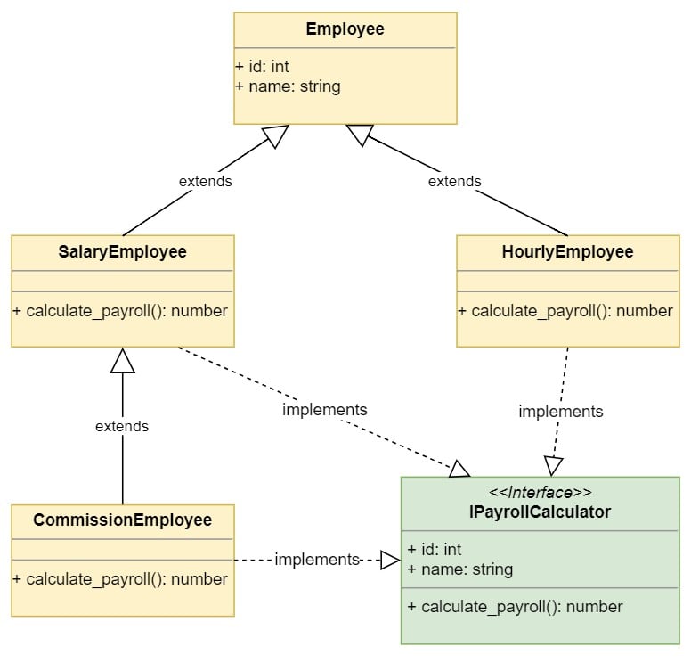
The diagram shows the inheritance hierarchy of the classes. The derived classes implement the IPayrollCalculator interface, which is required by the PayrollSystem. The PayrollSystem.calculate_payroll() implementation requires that the employee objects passed contain an id, name, and calculate_payroll() implementation.
Interfaces are represented similarly to classes with the word interface above the interface name. Interface names are usually prefixed with a capital I.
The application creates its employees and passes them to the payroll system to process payroll:
# In program.py
import hr
salary_employee = hr.SalaryEmployee(1, 'John Smith', 1500)
hourly_employee = hr.HourlyEmployee(2, 'Jane Doe', 40, 15)
commission_employee = hr.CommissionEmployee(3, 'Kevin Bacon', 1000, 250)
payroll_system = hr.PayrollSystem()
payroll_system.calculate_payroll([
salary_employee,
hourly_employee,
commission_employee
])
You can run the program in the command line and see the results:
$ python program.py
Calculating Payroll
===================
Payroll for: 1 - John Smith
- Check amount: 1500
Payroll for: 2 - Jane Doe
- Check amount: 600
Payroll for: 3 - Kevin Bacon
- Check amount: 1250
The program creates three employee objects, one for each of the derived classes. Then, it creates the payroll system and passes a list of the employees to its .calculate_payroll() method, which calculates the payroll for each employee and prints the results.
Notice how the Employee base class doesn’t define a .calculate_payroll() method. This means that if you were to create a plain Employee object and pass it to the PayrollSystem, then you’d get an error. You can try it in the Python interactive interpreter:
>>> import hr
>>> employee = hr.Employee(1, 'Invalid')
>>> payroll_system = hr.PayrollSystem()
>>> payroll_system.calculate_payroll([employee])
Payroll for: 1 - Invalid
Traceback (most recent call last):
File "<stdin>", line 1, in <module>
File "/hr.py", line 39, in calculate_payroll
print(f'- Check amount: {employee.calculate_payroll()}')
AttributeError: 'Employee' object has no attribute 'calculate_payroll'
While you can instantiate an Employee object, the object can’t be used by the PayrollSystem. Why? Because it can’t .calculate_payroll() for an Employee. To meet the requirements of PayrollSystem, you’ll want to convert the Employee class, which is currently a concrete class, to an abstract class. That way, no employee is ever just an Employee, but one that implements .calculate_payroll().
The Employee class in the example above is what is called an abstract base class. Abstract base classes exist to be inherited, but never instantiated. Python provides the abc module to define abstract base classes.
You can use leading underscores in your class name to communicate that objects of that class should not be created. Underscores provide a friendly way to prevent misuse of your code, but they don’t prevent eager users from creating instances of that class.
The abc module in the Python standard library provides functionality to prevent creating objects from abstract base classes.
You can modify the implementation of the Employee class to ensure that it can’t be instantiated:
# In hr.py
from abc import ABC, abstractmethod
class Employee(ABC):
def __init__(self, id, name):
self.id = id
self.name = name
@abstractmethod
def calculate_payroll(self):
pass
You derive Employee from ABC, making it an abstract base class. Then, you decorate the .calculate_payroll() method with the @abstractmethod decorator.
This change has two nice side-effects:
Employee can’t be created. hr module that if they derive from Employee, then they must override the .calculate_payroll() abstract method.You can see that objects of type Employee can’t be created using the interactive interpreter:
>>> import hr
>>> employee = hr.Employee(1, 'abstract')
Traceback (most recent call last):
File "<stdin>", line 1, in <module>
TypeError: Can't instantiate abstract class Employee with abstract methods
calculate_payroll
The output shows that the class cannot be instantiated because it contains an abstract method calculate_payroll(). Derived classes must override the method to allow creating objects of their type.
When you derive one class from another, the derived class inherits both:
The base class interface: The derived class inherits all the methods, properties, and attributes of the base class.
The base class implementation: The derived class inherits the code that implements the class interface.
Most of the time, you’ll want to inherit the implementation of a class, but you will want to implement multiple interfaces, so your objects can be used in different situations.
Modern programming languages are designed with this basic concept in mind. They allow you to inherit from a single class, but you can implement multiple interfaces.
In Python, you don’t have to explicitly declare an interface. Any object that implements the desired interface can be used in place of another object. This is known as duck typing. Duck typing is usually explained as “if it behaves like a duck, then it’s a duck.”
To illustrate this, you will now add a DisgruntledEmployee class to the example above which doesn’t derive from Employee:
# In disgruntled.py
class DisgruntledEmployee:
def __init__(self, id, name):
self.id = id
self.name = name
def calculate_payroll(self):
return 1000000
The DisgruntledEmployee class doesn’t derive from Employee, but it exposes the same interface required by the PayrollSystem. The PayrollSystem.calculate_payroll() requires a list of objects that implement the following interface:
id property or attribute that returns the employee’s idname property or attribute that represents the employee’s name.calculate_payroll() method that doesn’t take any parameters and returns the payroll amount to processAll these requirements are met by the DisgruntledEmployee class, so the PayrollSystem can still calculate its payroll.
You can modify the program to use the DisgruntledEmployee class:
# In program.py
import hr
import disgruntled
salary_employee = hr.SalaryEmployee(1, 'John Smith', 1500)
hourly_employee = hr.HourlyEmployee(2, 'Jane Doe', 40, 15)
commission_employee = hr.CommissionEmployee(3, 'Kevin Bacon', 1000, 250)
disgruntled_employee = disgruntled.DisgruntledEmployee(20000, 'Anonymous')
payroll_system = hr.PayrollSystem()
payroll_system.calculate_payroll([
salary_employee,
hourly_employee,
commission_employee,
disgruntled_employee
])
The program creates a DisgruntledEmployee object and adds it to the list processed by the PayrollSystem. You can now run the program and see its output:
$ python program.py
Calculating Payroll
===================
Payroll for: 1 - John Smith
- Check amount: 1500
Payroll for: 2 - Jane Doe
- Check amount: 600
Payroll for: 3 - Kevin Bacon
- Check amount: 1250
Payroll for: 20000 - Anonymous
- Check amount: 1000000
As you can see, the PayrollSystem can still process the new object because it meets the desired interface.
Since you don’t have to derive from a specific class for your objects to be reusable by the program, you may be asking why you should use inheritance instead of just implementing the desired interface. The following rules may help you:
Use inheritance to reuse an implementation: Your derived classes should leverage most of their base class implementation. They must also model an is a relationship. A Customer class might also have an id and a name, but a Customer is not an Employee, so you should not use inheritance.
Implement an interface to be reused: When you want your class to be reused by a specific part of your application, you implement the required interface in your class, but you don’t need to provide a base class, or inherit from another class.
You can now clean up the example above to move onto the next topic. You can delete the disgruntled.py file and then modify the hr module to its original state:
# In hr.py
class PayrollSystem:
def calculate_payroll(self, employees):
print('Calculating Payroll')
print('===================')
for employee in employees:
print(f'Payroll for: {employee.id} - {employee.name}')
print(f'- Check amount: {employee.calculate_payroll()}')
print('')
class Employee:
def __init__(self, id, name):
self.id = id
self.name = name
class SalaryEmployee(Employee):
def __init__(self, id, name, weekly_salary):
super().__init__(id, name)
self.weekly_salary = weekly_salary
def calculate_payroll(self):
return self.weekly_salary
class HourlyEmployee(Employee):
def __init__(self, id, name, hours_worked, hour_rate):
super().__init__(id, name)
self.hours_worked = hours_worked
self.hour_rate = hour_rate
def calculate_payroll(self):
return self.hours_worked * self.hour_rate
class CommissionEmployee(SalaryEmployee):
def __init__(self, id, name, weekly_salary, commission):
super().__init__(id, name, weekly_salary)
self.commission = commission
def calculate_payroll(self):
fixed = super().calculate_payroll()
return fixed + self.commission
You removed the import of the abc module since the Employee class doesn’t need to be abstract. You also removed the abstract calculate_payroll() method from it since it doesn’t provide any implementation.
Basically, you are inheriting the implementation of the id and name attributes of the Employee class in your derived classes. Since .calculate_payroll() is just an interface to the PayrollSystem.calculate_payroll() method, you don’t need to implement it in the Employee base class.
Notice how the CommissionEmployee class derives from SalaryEmployee. This means that CommissionEmployee inherits the implementation and interface of SalaryEmployee. You can see how the CommissionEmployee.calculate_payroll() method leverages the base class implementation because it relies on the result from super().calculate_payroll() to implement its own version.
If you are not careful, inheritance can lead you to a huge hierarchical structure of classes that is hard to understand and maintain. This is known as the class explosion problem.
You started building a class hierarchy of Employee types used by the PayrollSystem to calculate payroll. Now, you need to add some functionality to those classes, so they can be used with the new ProductivitySystem.
The ProductivitySystem tracks productivity based on employee roles. There are different employee roles:
With those requirements, you start to see that Employee and its derived classes might belong somewhere other than the hr module because now they’re also used by the ProductivitySystem.
You create an employees module and move the classes there:
# In employees.py
class Employee:
def __init__(self, id, name):
self.id = id
self.name = name
class SalaryEmployee(Employee):
def __init__(self, id, name, weekly_salary):
super().__init__(id, name)
self.weekly_salary = weekly_salary
def calculate_payroll(self):
return self.weekly_salary
class HourlyEmployee(Employee):
def __init__(self, id, name, hours_worked, hour_rate):
super().__init__(id, name)
self.hours_worked = hours_worked
self.hour_rate = hour_rate
def calculate_payroll(self):
return self.hours_worked * self.hour_rate
class CommissionEmployee(SalaryEmployee):
def __init__(self, id, name, weekly_salary, commission):
super().__init__(id, name, weekly_salary)
self.commission = commission
def calculate_payroll(self):
fixed = super().calculate_payroll()
return fixed + self.commission
The implementation remains the same, but you move the classes to the employee module. Now, you change your program to support the change:
# In program.py
import hr
import employees
salary_employee = employees.SalaryEmployee(1, 'John Smith', 1500)
hourly_employee = employees.HourlyEmployee(2, 'Jane Doe', 40, 15)
commission_employee = employees.CommissionEmployee(3, 'Kevin Bacon', 1000, 250)
payroll_system = hr.PayrollSystem()
payroll_system.calculate_payroll([
salary_employee,
hourly_employee,
commission_employee
])
You run the program and verify that it still works:
$ python program.py
Calculating Payroll
===================
Payroll for: 1 - John Smith
- Check amount: 1500
Payroll for: 2 - Jane Doe
- Check amount: 600
Payroll for: 3 - Kevin Bacon
- Check amount: 1250
With everything in place, you start adding the new classes:
# In employees.py
class Manager(SalaryEmployee):
def work(self, hours):
print(f'{self.name} screams and yells for {hours} hours.')
class Secretary(SalaryEmployee):
def work(self, hours):
print(f'{self.name} expends {hours} hours doing office paperwork.')
class SalesPerson(CommissionEmployee):
def work(self, hours):
print(f'{self.name} expends {hours} hours on the phone.')
class FactoryWorker(HourlyEmployee):
def work(self, hours):
print(f'{self.name} manufactures gadgets for {hours} hours.')
First, you add a Manager class that derives from SalaryEmployee. The class exposes a method work() that will be used by the productivity system. The method takes the hours the employee worked.
Then you add Secretary, SalesPerson, and FactoryWorker and then implement the work() interface, so they can be used by the productivity system.
Now, you can add the ProductivitySytem class:
# In productivity.py
class ProductivitySystem:
def track(self, employees, hours):
print('Tracking Employee Productivity')
print('==============================')
for employee in employees:
employee.work(hours)
print('')
The class tracks employees in the track() method that takes a list of employees and the number of hours to track. You can now add the productivity system to your program:
# In program.py
import hr
import employees
import productivity
manager = employees.Manager(1, 'Mary Poppins', 3000)
secretary = employees.Secretary(2, 'John Smith', 1500)
sales_guy = employees.SalesPerson(3, 'Kevin Bacon', 1000, 250)
factory_worker = employees.FactoryWorker(2, 'Jane Doe', 40, 15)
employees = [
manager,
secretary,
sales_guy,
factory_worker,
]
productivity_system = productivity.ProductivitySystem()
productivity_system.track(employees, 40)
payroll_system = hr.PayrollSystem()
payroll_system.calculate_payroll(employees)
The program creates a list of employees of different types. The employee list is sent to the productivity system to track their work for 40 hours. Then the same list of employees is sent to the payroll system to calculate their payroll.
You can run the program to see the output:
$ python program.py
Tracking Employee Productivity
==============================
Mary Poppins screams and yells for 40 hours.
John Smith expends 40 hours doing office paperwork.
Kevin Bacon expends 40 hours on the phone.
Jane Doe manufactures gadgets for 40 hours.
Calculating Payroll
===================
Payroll for: 1 - Mary Poppins
- Check amount: 3000
Payroll for: 2 - John Smith
- Check amount: 1500
Payroll for: 3 - Kevin Bacon
- Check amount: 1250
Payroll for: 4 - Jane Doe
- Check amount: 600
The program shows the employees working for 40 hours through the productivity system. Then it calculates and displays the payroll for each of the employees.
The program works as expected, but you had to add four new classes to support the changes. As new requirements come, your class hierarchy will inevitably grow, leading to the class explosion problem where your hierarchies will become so big that they’ll be hard to understand and maintain.
The following diagram shows the new class hierarchy:
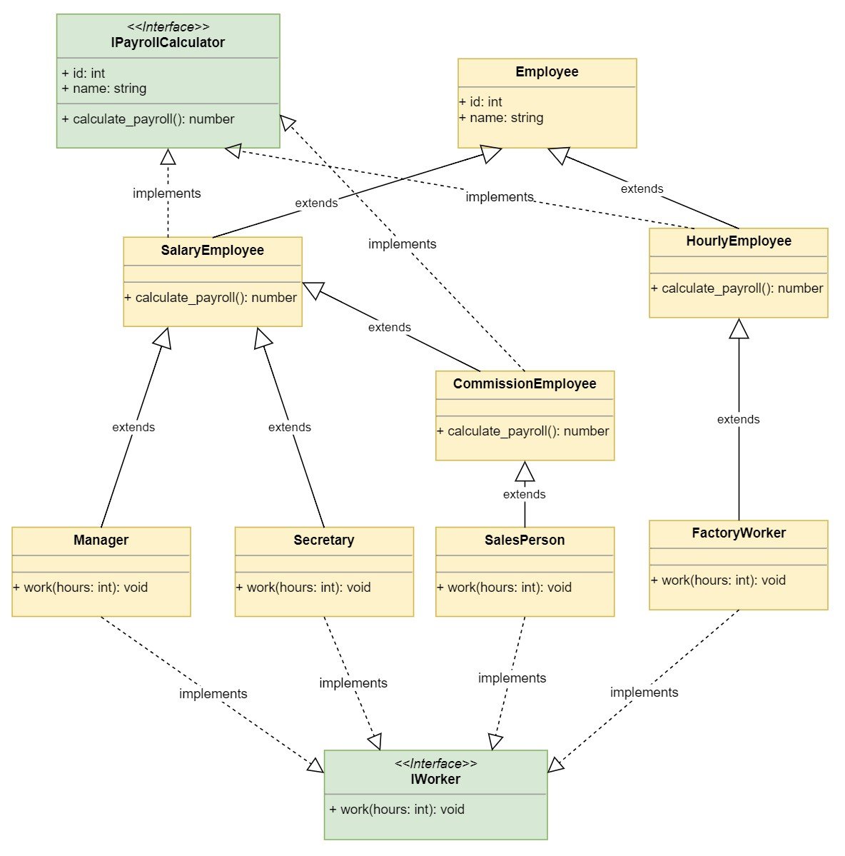
The diagram shows how the class hierarchy is growing. Additional requirements might have an exponential effect in the number of classes with this design.
Python is one of the few modern programming languages that supports multiple inheritance. Multiple inheritance is the ability to derive a class from multiple base classes at the same time.
Multiple inheritance has a bad reputation to the extent that most modern programming languages don’t support it. Instead, modern programming languages support the concept of interfaces. In those languages, you inherit from a single base class and then implement multiple interfaces, so your class can be re-used in different situations.
This approach puts some constraints in your designs. You can only inherit the implementation of one class by directly deriving from it. You can implement multiple interfaces, but you can’t inherit the implementation of multiple classes.
This constraint is good for software design because it forces you to design your classes with fewer dependencies on each other. You will see later in this article that you can leverage multiple implementations through composition, which makes software more flexible. This section, however, is about multiple inheritance, so let’s take a look at how it works.
It turns out that sometimes temporary secretaries are hired when there is too much paperwork to do. The TemporarySecretary class performs the role of a Secretary in the context of the ProductivitySystem, but for payroll purposes, it is an HourlyEmployee.
You look at your class design. It has grown a little bit, but you can still understand how it works. It seems you have two options:
Derive from Secretary: You can derive from Secretary to inherit the .work() method for the role, and then override the .calculate_payroll() method to implement it as an HourlyEmployee.
Derive from HourlyEmployee: You can derive from HourlyEmployee to inherit the .calculate_payroll() method, and then override the .work() method to implement it as a Secretary.
Then, you remember that Python supports multiple inheritance, so you decide to derive from both Secretary and HourlyEmployee:
# In employees.py
class TemporarySecretary(Secretary, HourlyEmployee):
pass
Python allows you to inherit from two different classes by specifying them between parenthesis in the class declaration.
Now, you modify your program to add the new temporary secretary employee:
import hr
import employees
import productivity
manager = employees.Manager(1, 'Mary Poppins', 3000)
secretary = employees.Secretary(2, 'John Smith', 1500)
sales_guy = employees.SalesPerson(3, 'Kevin Bacon', 1000, 250)
factory_worker = employees.FactoryWorker(4, 'Jane Doe', 40, 15)
temporary_secretary = employees.TemporarySecretary(5, 'Robin Williams', 40, 9)
company_employees = [
manager,
secretary,
sales_guy,
factory_worker,
temporary_secretary,
]
productivity_system = productivity.ProductivitySystem()
productivity_system.track(company_employees, 40)
payroll_system = hr.PayrollSystem()
payroll_system.calculate_payroll(company_employees)
You run the program to test it:
$ python program.py
Traceback (most recent call last):
File ".\program.py", line 9, in <module>
temporary_secretary = employee.TemporarySecretary(5, 'Robin Williams', 40, 9)
TypeError: __init__() takes 4 positional arguments but 5 were given
You get a TypeError exception saying that 4 positional arguments where expected, but 5 were given.
This is because you derived TemporarySecretary first from Secretary and then from HourlyEmployee, so the interpreter is trying to use Secretary.__init__() to initialize the object.
Okay, let’s reverse it:
class TemporarySecretary(HourlyEmployee, Secretary):
pass
Now, run the program again and see what happens:
$ python program.py
Traceback (most recent call last):
File ".\program.py", line 9, in <module>
temporary_secretary = employee.TemporarySecretary(5, 'Robin Williams', 40, 9)
File "employee.py", line 16, in __init__
super().__init__(id, name)
TypeError: __init__() missing 1 required positional argument: 'weekly_salary'
Now it seems you are missing a weekly_salary parameter, which is necessary to initialize Secretary, but that parameter doesn’t make sense in the context of a TemporarySecretary because it’s an HourlyEmployee.
Maybe implementing TemporarySecretary.__init__() will help:
# In employees.py
class TemporarySecretary(HourlyEmployee, Secretary):
def __init__(self, id, name, hours_worked, hour_rate):
super().__init__(id, name, hours_worked, hour_rate)
Try it:
$ python program.py
Traceback (most recent call last):
File ".\program.py", line 9, in <module>
temporary_secretary = employee.TemporarySecretary(5, 'Robin Williams', 40, 9)
File "employee.py", line 54, in __init__
super().__init__(id, name, hours_worked, hour_rate)
File "employee.py", line 16, in __init__
super().__init__(id, name)
TypeError: __init__() missing 1 required positional argument: 'weekly_salary'
That didn’t work either. Okay, it’s time for you to dive into Python’s method resolution order (MRO) to see what’s going on.
When a method or attribute of a class is accessed, Python uses the class MRO to find it. The MRO is also used by super() to determine which method or attribute to invoke. You can learn more about super() in Supercharge Your Classes With Python super().
You can evaluate the TemporarySecretary class MRO using the interactive interpreter:
>>> from employees import TemporarySecretary
>>> TemporarySecretary.__mro__
(<class 'employees.TemporarySecretary'>,
<class 'employees.HourlyEmployee'>,
<class 'employees.Secretary'>,
<class 'employees.SalaryEmployee'>,
<class 'employees.Employee'>,
<class 'object'>
)
The MRO shows the order in which Python is going to look for a matching attribute or method. In the example, this is what happens when we create the TemporarySecretary object:
The TemporarySecretary.__init__(self, id, name, hours_worked, hour_rate) method is called.
The super().__init__(id, name, hours_worked, hour_rate) call matches HourlyEmployee.__init__(self, id, name, hour_worked, hour_rate).
HourlyEmployee calls super().__init__(id, name), which the MRO is going to match to Secretary.__init__(), which is inherited from SalaryEmployee.__init__(self, id, name, weekly_salary).
Because the parameters don’t match, a TypeError exception is raised.
You can bypass the MRO by reversing the inheritance order and directly calling HourlyEmployee.__init__() as follows:
class TemporarySecretary(Secretary, HourlyEmployee):
def __init__(self, id, name, hours_worked, hour_rate):
HourlyEmployee.__init__(self, id, name, hours_worked, hour_rate)
That solves the problem of creating the object, but you will run into a similar problem when trying to calculate payroll. You can run the program to see the problem:
$ python program.py
Tracking Employee Productivity
==============================
Mary Poppins screams and yells for 40 hours.
John Smith expends 40 hours doing office paperwork.
Kevin Bacon expends 40 hours on the phone.
Jane Doe manufactures gadgets for 40 hours.
Robin Williams expends 40 hours doing office paperwork.
Calculating Payroll
===================
Payroll for: 1 - Mary Poppins
- Check amount: 3000
Payroll for: 2 - John Smith
- Check amount: 1500
Payroll for: 3 - Kevin Bacon
- Check amount: 1250
Payroll for: 4 - Jane Doe
- Check amount: 600
Payroll for: 5 - Robin Williams
Traceback (most recent call last):
File ".\program.py", line 20, in <module>
payroll_system.calculate_payroll(employees)
File "hr.py", line 7, in calculate_payroll
print(f'- Check amount: {employee.calculate_payroll()}')
File "employee.py", line 12, in calculate_payroll
return self.weekly_salary
AttributeError: 'TemporarySecretary' object has no attribute 'weekly_salary'
The problem now is that because you reversed the inheritance order, the MRO is finding the .calculate_payroll() method of SalariedEmployee before the one in HourlyEmployee. You need to override .calculate_payroll() in TemporarySecretary and invoke the right implementation from it:
class TemporarySecretary(Secretary, HourlyEmployee):
def __init__(self, id, name, hours_worked, hour_rate):
HourlyEmployee.__init__(self, id, name, hours_worked, hour_rate)
def calculate_payroll(self):
return HourlyEmployee.calculate_payroll(self)
The calculate_payroll() method directly invokes HourlyEmployee.calculate_payroll() to ensure that you get the correct result. You can run the program again to see it working:
$ python program.py
Tracking Employee Productivity
==============================
Mary Poppins screams and yells for 40 hours.
John Smith expends 40 hours doing office paperwork.
Kevin Bacon expends 40 hours on the phone.
Jane Doe manufactures gadgets for 40 hours.
Robin Williams expends 40 hours doing office paperwork.
Calculating Payroll
===================
Payroll for: 1 - Mary Poppins
- Check amount: 3000
Payroll for: 2 - John Smith
- Check amount: 1500
Payroll for: 3 - Kevin Bacon
- Check amount: 1250
Payroll for: 4 - Jane Doe
- Check amount: 600
Payroll for: 5 - Robin Williams
- Check amount: 360
The program now works as expected because you’re forcing the method resolution order by explicitly telling the interpreter which method we want to use.
As you can see, multiple inheritance can be confusing, especially when you run into the diamond problem.
The following diagram shows the diamond problem in your class hierarchy:
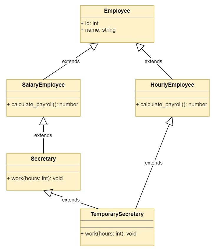
The diagram shows the diamond problem with the current class design. TemporarySecretary uses multiple inheritance to derive from two classes that ultimately also derive from Employee. This causes two paths to reach the Employee base class, which is something you want to avoid in your designs.
The diamond problem appears when you’re using multiple inheritance and deriving from two classes that have a common base class. This can cause the wrong version of a method to be called.
As you’ve seen, Python provides a way to force the right method to be invoked, and analyzing the MRO can help you understand the problem.
Still, when you run into the diamond problem, it’s better to re-think the design. You will now make some changes to leverage multiple inheritance, avoiding the diamond problem.
The Employee derived classes are used by two different systems:
The productivity system that tracks employee productivity.
The payroll system that calculates the employee payroll.
This means that everything related to productivity should be together in one module and everything related to payroll should be together in another. You can start making changes to the productivity module:
# In productivity.py
class ProductivitySystem:
def track(self, employees, hours):
print('Tracking Employee Productivity')
print('==============================')
for employee in employees:
result = employee.work(hours)
print(f'{employee.name}: {result}')
print('')
class ManagerRole:
def work(self, hours):
return f'screams and yells for {hours} hours.'
class SecretaryRole:
def work(self, hours):
return f'expends {hours} hours doing office paperwork.'
class SalesRole:
def work(self, hours):
return f'expends {hours} hours on the phone.'
class FactoryRole:
def work(self, hours):
return f'manufactures gadgets for {hours} hours.'
The productivity module implements the ProductivitySystem class, as well as the related roles it supports. The classes implement the work() interface required by the system, but they don’t derived from Employee.
You can do the same with the hr module:
# In hr.py
class PayrollSystem:
def calculate_payroll(self, employees):
print('Calculating Payroll')
print('===================')
for employee in employees:
print(f'Payroll for: {employee.id} - {employee.name}')
print(f'- Check amount: {employee.calculate_payroll()}')
print('')
class SalaryPolicy:
def __init__(self, weekly_salary):
self.weekly_salary = weekly_salary
def calculate_payroll(self):
return self.weekly_salary
class HourlyPolicy:
def __init__(self, hours_worked, hour_rate):
self.hours_worked = hours_worked
self.hour_rate = hour_rate
def calculate_payroll(self):
return self.hours_worked * self.hour_rate
class CommissionPolicy(SalaryPolicy):
def __init__(self, weekly_salary, commission):
super().__init__(weekly_salary)
self.commission = commission
def calculate_payroll(self):
fixed = super().calculate_payroll()
return fixed + self.commission
The hr module implements the PayrollSystem, which calculates payroll for the employees. It also implements the policy classes for payroll. As you can see, the policy classes don’t derive from Employee anymore.
You can now add the necessary classes to the employee module:
# In employees.py
from hr import (
SalaryPolicy,
CommissionPolicy,
HourlyPolicy
)
from productivity import (
ManagerRole,
SecretaryRole,
SalesRole,
FactoryRole
)
class Employee:
def __init__(self, id, name):
self.id = id
self.name = name
class Manager(Employee, ManagerRole, SalaryPolicy):
def __init__(self, id, name, weekly_salary):
SalaryPolicy.__init__(self, weekly_salary)
super().__init__(id, name)
class Secretary(Employee, SecretaryRole, SalaryPolicy):
def __init__(self, id, name, weekly_salary):
SalaryPolicy.__init__(self, weekly_salary)
super().__init__(id, name)
class SalesPerson(Employee, SalesRole, CommissionPolicy):
def __init__(self, id, name, weekly_salary, commission):
CommissionPolicy.__init__(self, weekly_salary, commission)
super().__init__(id, name)
class FactoryWorker(Employee, FactoryRole, HourlyPolicy):
def __init__(self, id, name, hours_worked, hour_rate):
HourlyPolicy.__init__(self, hours_worked, hour_rate)
super().__init__(id, name)
class TemporarySecretary(Employee, SecretaryRole, HourlyPolicy):
def __init__(self, id, name, hours_worked, hour_rate):
HourlyPolicy.__init__(self, hours_worked, hour_rate)
super().__init__(id, name)
The employees module imports policies and roles from the other modules and implements the different Employee types. You are still using multiple inheritance to inherit the implementation of the salary policy classes and the productivity roles, but the implementation of each class only needs to deal with initialization.
Notice that you still need to explicitly initialize the salary policies in the constructors. You probably saw that the initializations of Manager and Secretary are identical. Also, the initializations of FactoryWorker and TemporarySecretary are the same.
You will not want to have this kind of code duplication in more complex designs, so you have to be careful when designing class hierarchies.
Here’s the UML diagram for the new design:
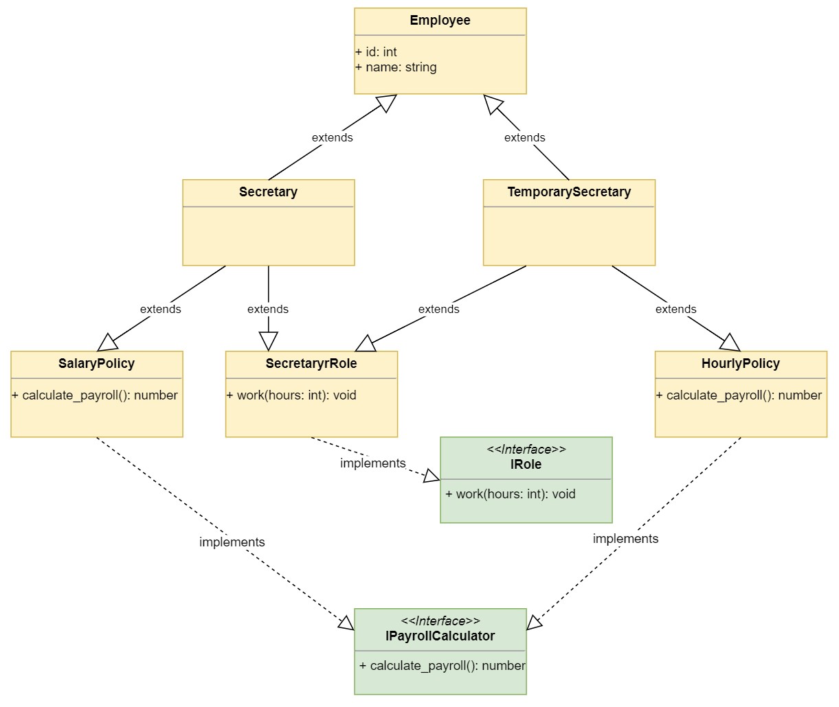
The diagram shows the relationships to define the Secretary and TemporarySecretary using multiple inheritance, but avoiding the diamond problem.
You can run the program and see how it works:
$ python program.py
Tracking Employee Productivity
==============================
Mary Poppins: screams and yells for 40 hours.
John Smith: expends 40 hours doing office paperwork.
Kevin Bacon: expends 40 hours on the phone.
Jane Doe: manufactures gadgets for 40 hours.
Robin Williams: expends 40 hours doing office paperwork.
Calculating Payroll
===================
Payroll for: 1 - Mary Poppins
- Check amount: 3000
Payroll for: 2 - John Smith
- Check amount: 1500
Payroll for: 3 - Kevin Bacon
- Check amount: 1250
Payroll for: 4 - Jane Doe
- Check amount: 600
Payroll for: 5 - Robin Williams
- Check amount: 360
You’ve seen how inheritance and multiple inheritance work in Python. You can now explore the topic of composition.
Composition is an object oriented design concept that models a has a relationship. In composition, a class known as composite contains an object of another class known to as component. In other words, a composite class has a component of another class.
Composition allows composite classes to reuse the implementation of the components it contains. The composite class doesn’t inherit the component class interface, but it can leverage its implementation.
The composition relation between two classes is considered loosely coupled. That means that changes to the component class rarely affect the composite class, and changes to the composite class never affect the component class.
This provides better adaptability to change and allows applications to introduce new requirements without affecting existing code.
When looking at two competing software designs, one based on inheritance and another based on composition, the composition solution usually is the most flexible. You can now look at how composition works.
You’ve already used composition in our examples. If you look at the Employee class, you’ll see that it contains two attributes:
id to identify an employee.name to contain the name of the employee.These two attributes are objects that the Employee class has. Therefore, you can say that an Employee has an id and has a name.
Another attribute for an Employee might be an Address:
# In contacts.py
class Address:
def __init__(self, street, city, state, zipcode, street2=''):
self.street = street
self.street2 = street2
self.city = city
self.state = state
self.zipcode = zipcode
def __str__(self):
lines = [self.street]
if self.street2:
lines.append(self.street2)
lines.append(f'{self.city}, {self.state} {self.zipcode}')
return '\n'.join(lines)
You implemented a basic address class that contains the usual components for an address. You made the street2 attribute optional because not all addresses will have that component.
You implemented __str__() to provide a pretty representation of an Address. You can see this implementation in the interactive interpreter:
>>> from contacts import Address
>>> address = Address('55 Main St.', 'Concord', 'NH', '03301')
>>> print(address)
55 Main St.
Concord, NH 03301
When you print() the address variable, the special method __str__() is invoked. Since you overloaded the method to return a string formatted as an address, you get a nice, readable representation. Operator and Function Overloading in Custom Python Classes gives a good overview of the special methods available in classes that can be implemented to customize the behavior of your objects.
You can now add the Address to the Employee class through composition:
# In employees.py
class Employee:
def __init__(self, id, name):
self.id = id
self.name = name
self.address = None
You initialize the address attribute to None for now to make it optional, but by doing that, you can now assign an Address to an Employee. Also notice that there is no reference in the employee module to the contacts module.
Composition is a loosely coupled relationship that often doesn’t require the composite class to have knowledge of the component.
The UML diagram representing the relationship between Employee and Address looks like this:
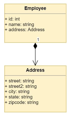
The diagram shows the basic composition relationship between Employee and Address.
You can now modify the PayrollSystem class to leverage the address attribute in Employee:
# In hr.py
class PayrollSystem:
def calculate_payroll(self, employees):
print('Calculating Payroll')
print('===================')
for employee in employees:
print(f'Payroll for: {employee.id} - {employee.name}')
print(f'- Check amount: {employee.calculate_payroll()}')
if employee.address:
print('- Sent to:')
print(employee.address)
print('')
You check to see if the employee object has an address, and if it does, you print it. You can now modify the program to assign some addresses to the employees:
# In program.py
import hr
import employees
import productivity
import contacts
manager = employees.Manager(1, 'Mary Poppins', 3000)
manager.address = contacts.Address(
'121 Admin Rd',
'Concord',
'NH',
'03301'
)
secretary = employees.Secretary(2, 'John Smith', 1500)
secretary.address = contacts.Address(
'67 Paperwork Ave.',
'Manchester',
'NH',
'03101'
)
sales_guy = employees.SalesPerson(3, 'Kevin Bacon', 1000, 250)
factory_worker = employees.FactoryWorker(4, 'Jane Doe', 40, 15)
temporary_secretary = employees.TemporarySecretary(5, 'Robin Williams', 40, 9)
employees = [
manager,
secretary,
sales_guy,
factory_worker,
temporary_secretary,
]
productivity_system = productivity.ProductivitySystem()
productivity_system.track(employees, 40)
payroll_system = hr.PayrollSystem()
payroll_system.calculate_payroll(employees)
You added a couple of addresses to the manager and secretary objects. When you run the program, you will see the addresses printed:
$ python program.py
Tracking Employee Productivity
==============================
Mary Poppins: screams and yells for {hours} hours.
John Smith: expends {hours} hours doing office paperwork.
Kevin Bacon: expends {hours} hours on the phone.
Jane Doe: manufactures gadgets for {hours} hours.
Robin Williams: expends {hours} hours doing office paperwork.
Calculating Payroll
===================
Payroll for: 1 - Mary Poppins
- Check amount: 3000
- Sent to:
121 Admin Rd
Concord, NH 03301
Payroll for: 2 - John Smith
- Check amount: 1500
- Sent to:
67 Paperwork Ave.
Manchester, NH 03101
Payroll for: 3 - Kevin Bacon
- Check amount: 1250
Payroll for: 4 - Jane Doe
- Check amount: 600
Payroll for: 5 - Robin Williams
- Check amount: 360
Notice how the payroll output for the manager and secretary objects show the addresses where the checks were sent.
The Employee class leverages the implementation of the Address class without any knowledge of what an Address object is or how it’s represented. This type of design is so flexible that you can change the Address class without any impact to the Employee class.
Composition is more flexible than inheritance because it models a loosely coupled relationship. Changes to a component class have minimal or no effects on the composite class. Designs based on composition are more suitable to change.
You change behavior by providing new components that implement those behaviors instead of adding new classes to your hierarchy.
Take a look at the multiple inheritance example above. Imagine how new payroll policies will affect the design. Try to picture what the class hierarchy will look like if new roles are needed. As you saw before, relying too heavily on inheritance can lead to class explosion.
The biggest problem is not so much the number of classes in your design, but how tightly coupled the relationships between those classes are. Tightly coupled classes affect each other when changes are introduced.
In this section, you are going to use composition to implement a better design that still fits the requirements of the PayrollSystem and the ProductivitySystem.
You can start by implementing the functionality of the ProductivitySystem:
# In productivity.py
class ProductivitySystem:
def __init__(self):
self._roles = {
'manager': ManagerRole,
'secretary': SecretaryRole,
'sales': SalesRole,
'factory': FactoryRole,
}
def get_role(self, role_id):
role_type = self._roles.get(role_id)
if not role_type:
raise ValueError('role_id')
return role_type()
def track(self, employees, hours):
print('Tracking Employee Productivity')
print('==============================')
for employee in employees:
employee.work(hours)
print('')
The ProductivitySystem class defines some roles using a string identifier mapped to a role class that implements the role. It exposes a .get_role() method that, given a role identifier, returns the role type object. If the role is not found, then a ValueError exception is raised.
It also exposes the previous functionality in the .track() method, where given a list of employees it tracks the productivity of those employees.
You can now implement the different role classes:
# In productivity.py
class ManagerRole:
def perform_duties(self, hours):
return f'screams and yells for {hours} hours.'
class SecretaryRole:
def perform_duties(self, hours):
return f'does paperwork for {hours} hours.'
class SalesRole:
def perform_duties(self, hours):
return f'expends {hours} hours on the phone.'
class FactoryRole:
def perform_duties(self, hours):
return f'manufactures gadgets for {hours} hours.'
Each of the roles you implemented expose a .perform_duties() that takes the number of hours worked. The methods return a string representing the duties.
The role classes are independent of each other, but they expose the same interface, so they are interchangeable. You’ll see later how they are used in the application.
Now, you can implement the PayrollSystem for the application:
# In hr.py
class PayrollSystem:
def __init__(self):
self._employee_policies = {
1: SalaryPolicy(3000),
2: SalaryPolicy(1500),
3: CommissionPolicy(1000, 100),
4: HourlyPolicy(15),
5: HourlyPolicy(9)
}
def get_policy(self, employee_id):
policy = self._employee_policies.get(employee_id)
if not policy:
return ValueError(employee_id)
return policy
def calculate_payroll(self, employees):
print('Calculating Payroll')
print('===================')
for employee in employees:
print(f'Payroll for: {employee.id} - {employee.name}')
print(f'- Check amount: {employee.calculate_payroll()}')
if employee.address:
print('- Sent to:')
print(employee.address)
print('')
The PayrollSystem keeps an internal database of payroll policies for each employee. It exposes a .get_policy() that, given an employee id, returns its payroll policy. If a specified id doesn’t exist in the system, then the method raises a ValueError exception.
The implementation of .calculate_payroll() works the same as before. It takes a list of employees, calculates the payroll, and prints the results.
You can now implement the payroll policy classes:
# In hr.py
class PayrollPolicy:
def __init__(self):
self.hours_worked = 0
def track_work(self, hours):
self.hours_worked += hours
class SalaryPolicy(PayrollPolicy):
def __init__(self, weekly_salary):
super().__init__()
self.weekly_salary = weekly_salary
def calculate_payroll(self):
return self.weekly_salary
class HourlyPolicy(PayrollPolicy):
def __init__(self, hour_rate):
super().__init__()
self.hour_rate = hour_rate
def calculate_payroll(self):
return self.hours_worked * self.hour_rate
class CommissionPolicy(SalaryPolicy):
def __init__(self, weekly_salary, commission_per_sale):
super().__init__(weekly_salary)
self.commission_per_sale = commission_per_sale
@property
def commission(self):
sales = self.hours_worked / 5
return sales * self.commission_per_sale
def calculate_payroll(self):
fixed = super().calculate_payroll()
return fixed + self.commission
You first implement a PayrollPolicy class that serves as a base class for all the payroll policies. This class tracks the hours_worked, which is common to all payroll policies.
The other policy classes derive from PayrollPolicy. We use inheritance here because we want to leverage the implementation of PayrollPolicy. Also, SalaryPolicy, HourlyPolicy, and CommissionPolicy are a PayrollPolicy.
SalaryPolicy is initialized with a weekly_salary value that is then used in .calculate_payroll(). HourlyPolicy is initialized with the hour_rate, and implements .calculate_payroll() by leveraging the base class hours_worked.
The CommissionPolicy class derives from SalaryPolicy because it wants to inherit its implementation. It is initialized with the weekly_salary parameters, but it also requires a commission_per_sale parameter.
The commission_per_sale is used to calculate the .commission, which is implemented as a property so it gets calculated when requested. In the example, we are assuming that a sale happens every 5 hours worked, and the .commission is the number of sales times the commission_per_sale value.
CommissionPolicy implements the .calculate_payroll() method by first leveraging the implementation in SalaryPolicy and then adding the calculated commission.
You can now add an AddressBook class to manage employee addresses:
# In contacts.py
class AddressBook:
def __init__(self):
self._employee_addresses = {
1: Address('121 Admin Rd.', 'Concord', 'NH', '03301'),
2: Address('67 Paperwork Ave', 'Manchester', 'NH', '03101'),
3: Address('15 Rose St', 'Concord', 'NH', '03301', 'Apt. B-1'),
4: Address('39 Sole St.', 'Concord', 'NH', '03301'),
5: Address('99 Mountain Rd.', 'Concord', 'NH', '03301'),
}
def get_employee_address(self, employee_id):
address = self._employee_addresses.get(employee_id)
if not address:
raise ValueError(employee_id)
return address
The AddressBook class keeps an internal database of Address objects for each employee. It exposes a get_employee_address() method that returns the address of the specified employee id. If the employee id doesn’t exist, then it raises a ValueError.
The Address class implementation remains the same as before:
# In contacts.py
class Address:
def __init__(self, street, city, state, zipcode, street2=''):
self.street = street
self.street2 = street2
self.city = city
self.state = state
self.zipcode = zipcode
def __str__(self):
lines = [self.street]
if self.street2:
lines.append(self.street2)
lines.append(f'{self.city}, {self.state} {self.zipcode}')
return '\n'.join(lines)
The class manages the address components and provides a pretty representation of an address.
So far, the new classes have been extended to support more functionality, but there are no significant changes to the previous design. This is going to change with the design of the employees module and its classes.
You can start by implementing an EmployeeDatabase class:
# In employees.py
from productivity import ProductivitySystem
from hr import PayrollSystem
from contacts import AddressBook
class EmployeeDatabase:
def __init__(self):
self._employees = [
{
'id': 1,
'name': 'Mary Poppins',
'role': 'manager'
},
{
'id': 2,
'name': 'John Smith',
'role': 'secretary'
},
{
'id': 3,
'name': 'Kevin Bacon',
'role': 'sales'
},
{
'id': 4,
'name': 'Jane Doe',
'role': 'factory'
},
{
'id': 5,
'name': 'Robin Williams',
'role': 'secretary'
},
]
self.productivity = ProductivitySystem()
self.payroll = PayrollSystem()
self.employee_addresses = AddressBook()
@property
def employees(self):
return [self._create_employee(**data) for data in self._employees]
def _create_employee(self, id, name, role):
address = self.employee_addresses.get_employee_address(id)
employee_role = self.productivity.get_role(role)
payroll_policy = self.payroll.get_policy(id)
return Employee(id, name, address, employee_role, payroll_policy)
The EmployeeDatabase keeps track of all the employees in the company. For each employee, it tracks the id, name, and role. It has an instance of the ProductivitySystem, the PayrollSystem, and the AddressBook. These instances are used to create employees.
It exposes an .employees property that returns the list of employees. The Employee objects are created in an internal method ._create_employee(). Notice that you don’t have different types of Employee classes. You just need to implement a single Employee class:
# In employees.py
class Employee:
def __init__(self, id, name, address, role, payroll):
self.id = id
self.name = name
self.address = address
self.role = role
self.payroll = payroll
def work(self, hours):
duties = self.role.perform_duties(hours)
print(f'Employee {self.id} - {self.name}:')
print(f'- {duties}')
print('')
self.payroll.track_work(hours)
def calculate_payroll(self):
return self.payroll.calculate_payroll()
The Employee class is initialized with the id, name, and address attributes. It also requires the productivity role for the employee and the payroll policy.
The class exposes a .work() method that takes the hours worked. This method first retrieves the duties from the role. In other words, it delegates to the role object to perform its duties.
In the same way, it delegates to the payroll object to track the work hours. The payroll, as you saw, uses those hours to calculate the payroll if needed.
The following diagram shows the composition design used:
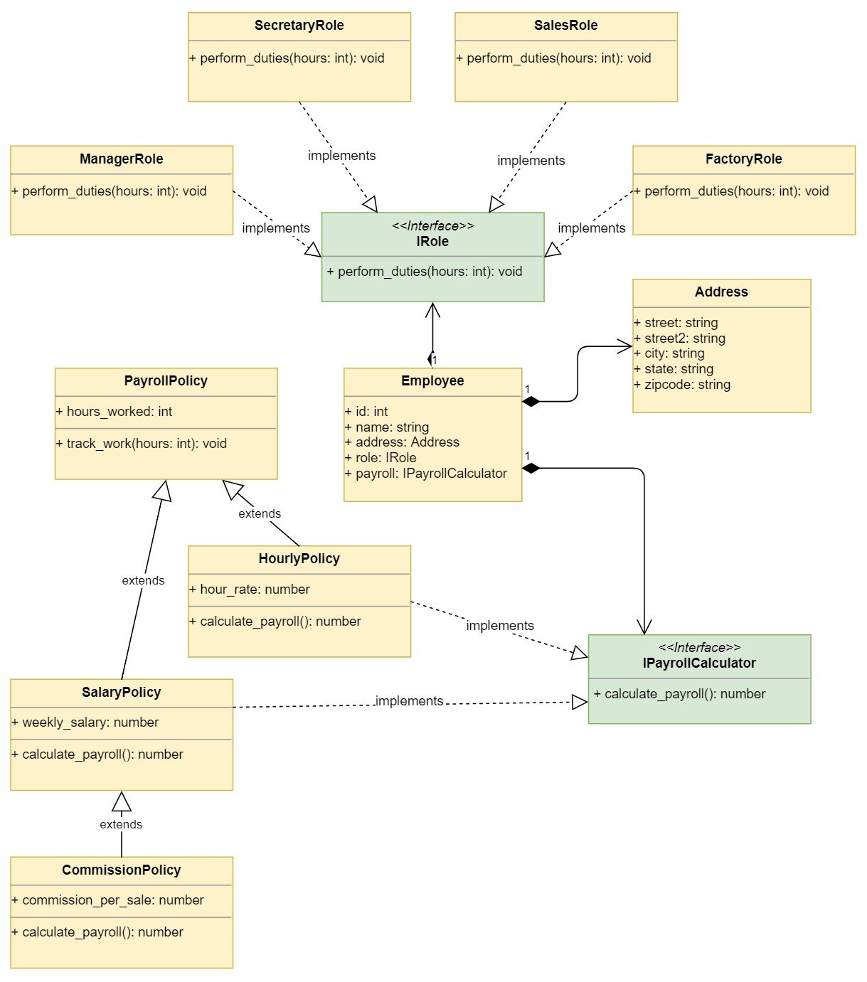
The diagram shows the design of composition based policies. There is a single Employee that is composed of other data objects like Address and depends on the IRole and IPayrollCalculator interfaces to delegate the work. There are multiple implementations of these interfaces.
You can now use this design in your program:
# In program.py
from hr import PayrollSystem
from productivity import ProductivitySystem
from employees import EmployeeDatabase
productivity_system = ProductivitySystem()
payroll_system = PayrollSystem()
employee_database = EmployeeDatabase()
employees = employee_database.employees
productivity_system.track(employees, 40)
payroll_system.calculate_payroll(employees)
You can run the program to see its output:
$ python program.py
Tracking Employee Productivity
==============================
Employee 1 - Mary Poppins:
- screams and yells for 40 hours.
Employee 2 - John Smith:
- does paperwork for 40 hours.
Employee 3 - Kevin Bacon:
- expends 40 hours on the phone.
Employee 4 - Jane Doe:
- manufactures gadgets for 40 hours.
Employee 5 - Robin Williams:
- does paperwork for 40 hours.
Calculating Payroll
===================
Payroll for: 1 - Mary Poppins
- Check amount: 3000
- Sent to:
121 Admin Rd.
Concord, NH 03301
Payroll for: 2 - John Smith
- Check amount: 1500
- Sent to:
67 Paperwork Ave
Manchester, NH 03101
Payroll for: 3 - Kevin Bacon
- Check amount: 1800.0
- Sent to:
15 Rose St
Apt. B-1
Concord, NH 03301
Payroll for: 4 - Jane Doe
- Check amount: 600
- Sent to:
39 Sole St.
Concord, NH 03301
Payroll for: 5 - Robin Williams
- Check amount: 360
- Sent to:
99 Mountain Rd.
Concord, NH 03301
This design is what is called policy-based design, where classes are composed of policies, and they delegate to those policies to do the work.
Policy-based design was introduced in the book Modern C++ Design, and it uses template metaprogramming in C++ to achieve the results.
Python does not support templates, but you can achieve similar results using composition, as you saw in the example above.
This type of design gives you all the flexibility you’ll need as requirements change. Imagine you need to change the way payroll is calculated for an object at run-time.
If your design relies on inheritance, you need to find a way to change the type of an object to change its behavior. With composition, you just need to change the policy the object uses.
Imagine that our manager all of a sudden becomes a temporary employee that gets paid by the hour. You can modify the object during the execution of the program in the following way:
# In program.py
from hr import PayrollSystem, HourlyPolicy
from productivity import ProductivitySystem
from employees import EmployeeDatabase
productivity_system = ProductivitySystem()
payroll_system = PayrollSystem()
employee_database = EmployeeDatabase()
employees = employee_database.employees
manager = employees[0]
manager.payroll = HourlyPolicy(55)
productivity_system.track(employees, 40)
payroll_system.calculate_payroll(employees)
The program gets the employee list from the EmployeeDatabase and retrieves the first employee, which is the manager we want. Then it creates a new HourlyPolicy initialized at $55 per hour and assigns it to the manager object.
The new policy is now used by the PayrollSystem modifying the existing behavior. You can run the program again to see the result:
$ python program.py
Tracking Employee Productivity
==============================
Employee 1 - Mary Poppins:
- screams and yells for 40 hours.
Employee 2 - John Smith:
- does paperwork for 40 hours.
Employee 3 - Kevin Bacon:
- expends 40 hours on the phone.
Employee 4 - Jane Doe:
- manufactures gadgets for 40 hours.
Employee 5 - Robin Williams:
- does paperwork for 40 hours.
Calculating Payroll
===================
Payroll for: 1 - Mary Poppins
- Check amount: 2200
- Sent to:
121 Admin Rd.
Concord, NH 03301
Payroll for: 2 - John Smith
- Check amount: 1500
- Sent to:
67 Paperwork Ave
Manchester, NH 03101
Payroll for: 3 - Kevin Bacon
- Check amount: 1800.0
- Sent to:
15 Rose St
Apt. B-1
Concord, NH 03301
Payroll for: 4 - Jane Doe
- Check amount: 600
- Sent to:
39 Sole St.
Concord, NH 03301
Payroll for: 5 - Robin Williams
- Check amount: 360
- Sent to:
99 Mountain Rd.
Concord, NH 03301
The check for Mary Poppins, our manager, is now for $2200 instead of the fixed salary of $3000 that she had per week.
Notice how we added that business rule to the program without changing any of the existing classes. Consider what type of changes would’ve been required with an inheritance design.
You would’ve had to create a new class and change the type of the manager employee. There is no chance you could’ve changed the policy at run-time.
So far, you’ve seen how inheritance and composition work in Python. You’ve seen that derived classes inherit the interface and implementation of their base classes. You’ve also seen that composition allows you to reuse the implementation of another class.
You’ve implemented two solutions to the same problem. The first solution used multiple inheritance, and the second one used composition.
You’ve also seen that Python’s duck typing allows you to reuse objects with existing parts of a program by implementing the desired interface. In Python, it isn’t necessary to derive from a base class for your classes to be reused.
At this point, you might be asking when to use inheritance vs composition in Python. They both enable code reuse. Inheritance and composition can tackle similar problems in your Python programs.
The general advice is to use the relationship that creates fewer dependencies between two classes. This relation is composition. Still, there will be times where inheritance will make more sense.
The following sections provide some guidelines to help you make the right choice between inheritance and composition in Python.
Inheritance should only be used to model an is a relationship. Liskov’s substitution principle says that an object of type Derived, which inherits from Base, can replace an object of type Base without altering the desirable properties of a program.
Liskov’s substitution principle is the most important guideline to determine if inheritance is the appropriate design solution. Still, the answer might not be straightforward in all situations. Fortunately, there is a simple test you can use to determine if your design follows Liskov’s substitution principle.
Let’s say you have a class A that provides an implementation and interface you want to reuse in another class B. Your initial thought is that you can derive B from A and inherit both the interface and implementation. To be sure this is the right design, you follow theses steps:
Evaluate B is an A: Think about this relationship and justify it. Does it make sense?
Evaluate A is a B: Reverse the relationship and justify it. Does it also make sense?
If you can justify both relationships, then you should never inherit those classes from one another. Let’s look at a more concrete example.
You have a class Rectangle which exposes an .area property. You need a class Square, which also has an .area. It seems that a Square is a special type of Rectangle, so maybe you can derive from it and leverage both the interface and implementation.
Before you jump into the implementation, you use Liskov’s substitution principle to evaluate the relationship.
A Square is a Rectangle because its area is calculated from the product of its height times its length. The constraint is that Square.height and Square.length must be equal.
It makes sense. You can justify the relationship and explain why a Square is a Rectangle. Let’s reverse the relationship to see if it makes sense.
A Rectangle is a Square because its area is calculated from the product of its height times its length. The difference is that Rectangle.height and Rectangle.width can change independently.
It also makes sense. You can justify the relationship and describe the special constraints for each class. This is a good sign that these two classes should never derive from each other.
You might have seen other examples that derive Square from Rectangle to explain inheritance. You might be skeptical with the little test you just did. Fair enough. Let’s write a program that illustrates the problem with deriving Square from Rectangle.
First, you implement Rectangle. You’re even going to encapsulate the attributes to ensure that all the constraints are met:
# In rectangle_square_demo.py
class Rectangle:
def __init__(self, length, height):
self._length = length
self._height = height
@property
def area(self):
return self._length * self._height
The Rectangle class is initialized with a length and a height, and it provides an .area property that returns the area. The length and height are encapsulated to avoid changing them directly.
Now, you derive Square from Rectangle and override the necessary interface to meet the constraints of a Square:
# In rectangle_square_demo.py
class Square(Rectangle):
def __init__(self, side_size):
super().__init__(side_size, side_size)
The Square class is initialized with a side_size, which is used to initialize both components of the base class. Now, you write a small program to test the behavior:
# In rectangle_square_demo.py
rectangle = Rectangle(2, 4)
assert rectangle.area == 8
square = Square(2)
assert square.area == 4
print('OK!')
The program creates a Rectangle and a Square and asserts that their .area is calculated correctly. You can run the program and see that everything is OK so far:
$ python rectangle_square_demo.py
OK!
The program executes correctly, so it seems that Square is just a special case of a Rectangle.
Later on, you need to support resizing Rectangle objects, so you make the appropriate changes to the class:
# In rectangle_square_demo.py
class Rectangle:
def __init__(self, length, height):
self._length = length
self._height = height
@property
def area(self):
return self._length * self._height
def resize(self, new_length, new_height):
self._length = new_length
self._height = new_height
.resize() takes the new_length and new_width for the object. You can add the following code to the program to verify that it works correctly:
# In rectangle_square_demo.py
rectangle.resize(3, 5)
assert rectangle.area == 15
print('OK!')
You resize the rectangle object and assert that the new area is correct. You can run the program to verify the behavior:
$ python rectangle_square_demo.py
OK!
The assertion passes, and you see that the program runs correctly.
So, what happens if you resize a square? Modify the program, and try to modify the square object:
# In rectangle_square_demo.py
square.resize(3, 5)
print(f'Square area: {square.area}')
You pass the same parameters to square.resize() that you used with rectangle, and print the area. When you run the program you see:
$ python rectangle_square_demo.py
Square area: 15
OK!
The program shows that the new area is 15 like the rectangle object. The problem now is that the square object no longer meets the Square class constraint that the length and height must be equal.
How can you fix that problem? You can try several approaches, but all of them will be awkward. You can override .resize() in square and ignore the height parameter, but that will be confusing for people looking at other parts of the program where rectangles are being resized and some of them are not getting the expected areas because they are really squares.
In a small program like this one, it might be easy to spot the causes of the weird behavior, but in a more complex program, the problem will be harder to find.
The reality is that if you’re able to justify an inheritance relationship between two classes both ways, you should not derive one class from another.
In the example, it doesn’t make sense that Square inherits the interface and implementation of .resize() from Rectangle. That doesn’t mean that Square objects can’t be resized. It means that the interface is different because it only needs a side_size parameter.
This difference in interface justifies not deriving Square from Rectangle like the test above advised.
One of the uses of multiple inheritance in Python is to extend a class features through mixins. A mixin is a class that provides methods to other classes but are not considered a base class.
A mixin allows other classes to reuse its interface and implementation without becoming a super class. They implement a unique behavior that can be aggregated to other unrelated classes. They are similar to composition but they create a stronger relationship.
Let’s say you want to convert objects of certain types in your application to a dictionary representation of the object. You could provide a .to_dict() method in every class that you want to support this feature, but the implementation of .to_dict() seems to be very similar.
This could be a good candidate for a mixin. You start by slightly modifying the Employee class from the composition example:
# In employees.py
class Employee:
def __init__(self, id, name, address, role, payroll):
self.id = id
self.name = name
self.address = address
self._role = role
self._payroll = payroll
def work(self, hours):
duties = self._role.perform_duties(hours)
print(f'Employee {self.id} - {self.name}:')
print(f'- {duties}')
print('')
self._payroll.track_work(hours)
def calculate_payroll(self):
return self._payroll.calculate_payroll()
The change is very small. You just changed the role and payroll attributes to be internal by adding a leading underscore to their name. You will see soon why you are making that change.
Now, you add the AsDictionaryMixin class:
# In representations.py
class AsDictionaryMixin:
def to_dict(self):
return {
prop: self._represent(value)
for prop, value in self.__dict__.items()
if not self._is_internal(prop)
}
def _represent(self, value):
if isinstance(value, object):
if hasattr(value, 'to_dict'):
return value.to_dict()
else:
return str(value)
else:
return value
def _is_internal(self, prop):
return prop.startswith('_')
The AsDictionaryMixin class exposes a .to_dict() method that returns the representation of itself as a dictionary. The method is implemented as a dict comprehension that says, “Create a dictionary mapping prop to value for each item in self.__dict__.items() if the prop is not internal.”
Note: This is why we made the role and payroll attributes internal in the Employee class, because we don’t want to represent them in the dictionary.
As you saw at the beginning, creating a class inherits some members from object, and one of those members is __dict__, which is basically a mapping of all the attributes in an object to their value.
You iterate through all the items in __dict__ and filter out the ones that have a name that starts with an underscore using ._is_internal().
._represent() checks the specified value. If the value is an object, then it looks to see if it also has a .to_dict() member and uses it to represent the object. Otherwise, it returns a string representation. If the value is not an object, then it simply returns the value.
You can modify the Employee class to support this mixin:
# In employees.py
from representations import AsDictionaryMixin
class Employee(AsDictionaryMixin):
def __init__(self, id, name, address, role, payroll):
self.id = id
self.name = name
self.address = address
self._role = role
self._payroll = payroll
def work(self, hours):
duties = self._role.perform_duties(hours)
print(f'Employee {self.id} - {self.name}:')
print(f'- {duties}')
print('')
self._payroll.track_work(hours)
def calculate_payroll(self):
return self._payroll.calculate_payroll()
All you have to do is inherit the AsDictionaryMixin to support the functionality. It will be nice to support the same functionality in the Address class, so the Employee.address attribute is represented in the same way:
# In contacts.py
from representations import AsDictionaryMixin
class Address(AsDictionaryMixin):
def __init__(self, street, city, state, zipcode, street2=''):
self.street = street
self.street2 = street2
self.city = city
self.state = state
self.zipcode = zipcode
def __str__(self):
lines = [self.street]
if self.street2:
lines.append(self.street2)
lines.append(f'{self.city}, {self.state} {self.zipcode}')
return '\n'.join(lines)
You apply the mixin to the Address class to support the feature. Now, you can write a small program to test it:
# In program.py
import json
from employees import EmployeeDatabase
def print_dict(d):
print(json.dumps(d, indent=2))
for employee in EmployeeDatabase().employees:
print_dict(employee.to_dict())
The program implements a print_dict() that converts the dictionary to a JSON string using indentation so the output looks better.
Then, it iterates through all the employees, printing the dictionary representation provided by .to_dict(). You can run the program to see its output:
$ python program.py
{
"id": "1",
"name": "Mary Poppins",
"address": {
"street": "121 Admin Rd.",
"street2": "",
"city": "Concord",
"state": "NH",
"zipcode": "03301"
}
}
{
"id": "2",
"name": "John Smith",
"address": {
"street": "67 Paperwork Ave",
"street2": "",
"city": "Manchester",
"state": "NH",
"zipcode": "03101"
}
}
{
"id": "3",
"name": "Kevin Bacon",
"address": {
"street": "15 Rose St",
"street2": "Apt. B-1",
"city": "Concord",
"state": "NH",
"zipcode": "03301"
}
}
{
"id": "4",
"name": "Jane Doe",
"address": {
"street": "39 Sole St.",
"street2": "",
"city": "Concord",
"state": "NH",
"zipcode": "03301"
}
}
{
"id": "5",
"name": "Robin Williams",
"address": {
"street": "99 Mountain Rd.",
"street2": "",
"city": "Concord",
"state": "NH",
"zipcode": "03301"
}
}
You leveraged the implementation of AsDictionaryMixin in both Employee and Address classes even when they are not related. Because AsDictionaryMixin only provides behavior, it is easy to reuse with other classes without causing problems.
Composition models a has a relationship. With composition, a class Composite has an instance of class Component and can leverage its implementation. The Component class can be reused in other classes completely unrelated to the Composite.
In the composition example above, the Employee class has an Address object. Address implements all the functionality to handle addresses, and it can be reused by other classes.
Other classes like Customer or Vendor can reuse Address without being related to Employee. They can leverage the same implementation ensuring that addresses are handled consistently across the application.
A problem you may run into when using composition is that some of your classes may start growing by using multiple components. Your classes may require multiple parameters in the constructor just to pass in the components they are made of. This can make your classes hard to use.
A way to avoid the problem is by using the Factory Method to construct your objects. You did that with the composition example.
If you look at the implementation of the EmployeeDatabase class, you’ll notice that it uses ._create_employee() to construct an Employee object with the right parameters.
This design will work, but ideally, you should be able to construct an Employee object just by specifying an id, for example employee = Employee(1).
The following changes might improve your design. You can start with the productivity module:
# In productivity.py
class _ProductivitySystem:
def __init__(self):
self._roles = {
'manager': ManagerRole,
'secretary': SecretaryRole,
'sales': SalesRole,
'factory': FactoryRole,
}
def get_role(self, role_id):
role_type = self._roles.get(role_id)
if not role_type:
raise ValueError('role_id')
return role_type()
def track(self, employees, hours):
print('Tracking Employee Productivity')
print('==============================')
for employee in employees:
employee.work(hours)
print('')
# Role classes implementation omitted
_productivity_system = _ProductivitySystem()
def get_role(role_id):
return _productivity_system.get_role(role_id)
def track(employees, hours):
_productivity_system.track(employees, hours)
First, you make the _ProductivitySystem class internal, and then provide a _productivity_system internal variable to the module. You are communicating to other developers that they should not create or use the _ProductivitySystem directly. Instead, you provide two functions, get_role() and track(), as the public interface to the module. This is what other modules should use.
What you are saying is that the _ProductivitySystem is a Singleton, and there should only be one object created from it.
Now, you can do the same with the hr module:
# In hr.py
class _PayrollSystem:
def __init__(self):
self._employee_policies = {
1: SalaryPolicy(3000),
2: SalaryPolicy(1500),
3: CommissionPolicy(1000, 100),
4: HourlyPolicy(15),
5: HourlyPolicy(9)
}
def get_policy(self, employee_id):
policy = self._employee_policies.get(employee_id)
if not policy:
return ValueError(employee_id)
return policy
def calculate_payroll(self, employees):
print('Calculating Payroll')
print('===================')
for employee in employees:
print(f'Payroll for: {employee.id} - {employee.name}')
print(f'- Check amount: {employee.calculate_payroll()}')
if employee.address:
print('- Sent to:')
print(employee.address)
print('')
# Policy classes implementation omitted
_payroll_system = _PayrollSystem()
def get_policy(employee_id):
return _payroll_system.get_policy(employee_id)
def calculate_payroll(employees):
_payroll_system.calculate_payroll(employees)
Again, you make the _PayrollSystem internal and provide a public interface to it. The application will use the public interface to get policies and calculate payroll.
You will now do the same with the contacts module:
# In contacts.py
class _AddressBook:
def __init__(self):
self._employee_addresses = {
1: Address('121 Admin Rd.', 'Concord', 'NH', '03301'),
2: Address('67 Paperwork Ave', 'Manchester', 'NH', '03101'),
3: Address('15 Rose St', 'Concord', 'NH', '03301', 'Apt. B-1'),
4: Address('39 Sole St.', 'Concord', 'NH', '03301'),
5: Address('99 Mountain Rd.', 'Concord', 'NH', '03301'),
}
def get_employee_address(self, employee_id):
address = self._employee_addresses.get(employee_id)
if not address:
raise ValueError(employee_id)
return address
# Implementation of Address class omitted
_address_book = _AddressBook()
def get_employee_address(employee_id):
return _address_book.get_employee_address(employee_id)
You are basically saying that there should only be one _AddressBook, one _PayrollSystem, and one _ProductivitySystem. Again, this design pattern is called the Singleton design pattern, which comes in handy for classes from which there should only be one, single instance.
Now, you can work on the employees module. You will also make a Singleton out of the _EmployeeDatabase, but you will make some additional changes:
# In employees.py
from productivity import get_role
from hr import get_policy
from contacts import get_employee_address
from representations import AsDictionaryMixin
class _EmployeeDatabase:
def __init__(self):
self._employees = {
1: {
'name': 'Mary Poppins',
'role': 'manager'
},
2: {
'name': 'John Smith',
'role': 'secretary'
},
3: {
'name': 'Kevin Bacon',
'role': 'sales'
},
4: {
'name': 'Jane Doe',
'role': 'factory'
},
5: {
'name': 'Robin Williams',
'role': 'secretary'
}
}
@property
def employees(self):
return [Employee(id_) for id_ in sorted(self._employees)]
def get_employee_info(self, employee_id):
info = self._employees.get(employee_id)
if not info:
raise ValueError(employee_id)
return info
class Employee(AsDictionaryMixin):
def __init__(self, id):
self.id = id
info = employee_database.get_employee_info(self.id)
self.name = info.get('name')
self.address = get_employee_address(self.id)
self._role = get_role(info.get('role'))
self._payroll = get_policy(self.id)
def work(self, hours):
duties = self._role.perform_duties(hours)
print(f'Employee {self.id} - {self.name}:')
print(f'- {duties}')
print('')
self._payroll.track_work(hours)
def calculate_payroll(self):
return self._payroll.calculate_payroll()
employee_database = _EmployeeDatabase()
You first import the relevant functions and classes from other modules. The _EmployeeDatabase is made internal, and at the bottom, you create a single instance. This instance is public and part of the interface because you will want to use it in the application.
You changed the _EmployeeDatabase._employees attribute to be a dictionary where the key is the employee id and the value is the employee information. You also exposed a .get_employee_info() method to return the information for the specified employee employee_id.
The _EmployeeDatabase.employees property now sorts the keys to return the employees sorted by their id. You replaced the method that constructed the Employee objects with calls to the Employee initializer directly.
The Employee class now is initialized with the id and uses the public functions exposed in the other modules to initialize its attributes.
You can now change the program to test the changes:
# In program.py
import json
from hr import calculate_payroll
from productivity import track
from employees import employee_database, Employee
def print_dict(d):
print(json.dumps(d, indent=2))
employees = employee_database.employees
track(employees, 40)
calculate_payroll(employees)
temp_secretary = Employee(5)
print('Temporary Secretary:')
print_dict(temp_secretary.to_dict())
You import the relevant functions from the hr and productivity modules, as well as the employee_database and Employee class. The program is cleaner because you exposed the required interface and encapsulated how objects are accessed.
Notice that you can now create an Employee object directly just using its id. You can run the program to see its output:
$ python program.py
Tracking Employee Productivity
==============================
Employee 1 - Mary Poppins:
- screams and yells for 40 hours.
Employee 2 - John Smith:
- does paperwork for 40 hours.
Employee 3 - Kevin Bacon:
- expends 40 hours on the phone.
Employee 4 - Jane Doe:
- manufactures gadgets for 40 hours.
Employee 5 - Robin Williams:
- does paperwork for 40 hours.
Calculating Payroll
===================
Payroll for: 1 - Mary Poppins
- Check amount: 3000
- Sent to:
121 Admin Rd.
Concord, NH 03301
Payroll for: 2 - John Smith
- Check amount: 1500
- Sent to:
67 Paperwork Ave
Manchester, NH 03101
Payroll for: 3 - Kevin Bacon
- Check amount: 1800.0
- Sent to:
15 Rose St
Apt. B-1
Concord, NH 03301
Payroll for: 4 - Jane Doe
- Check amount: 600
- Sent to:
39 Sole St.
Concord, NH 03301
Payroll for: 5 - Robin Williams
- Check amount: 360
- Sent to:
99 Mountain Rd.
Concord, NH 03301
Temporary Secretary:
{
"id": "5",
"name": "Robin Williams",
"address": {
"street": "99 Mountain Rd.",
"street2": "",
"city": "Concord",
"state": "NH",
"zipcode": "03301"
}
}
The program works the same as before, but now you can see that a single Employee object can be created from its id and display its dictionary representation.
Take a closer look at the Employee class:
# In employees.py
class Employee(AsDictionaryMixin):
def __init__(self, id):
self.id = id
info = employee_database.get_employee_info(self.id)
self.name = info.get('name')
self.address = get_employee_address(self.id)
self._role = get_role(info.get('role'))
self._payroll = get_policy(self.id)
def work(self, hours):
duties = self._role.perform_duties(hours)
print(f'Employee {self.id} - {self.name}:')
print(f'- {duties}')
print('')
self._payroll.track_work(hours)
def calculate_payroll(self):
return self._payroll.calculate_payroll()
The Employee class is a composite that contains multiple objects providing different functionality. It contains an Address that implements all the functionality related to where the employee lives.
Employee also contains a productivity role provided by the productivity module, and a payroll policy provided by the hr module. These two objects provide implementations that are leveraged by the Employee class to track work in the .work() method and to calculate the payroll in the .calculate_payroll() method.
You are using composition in two different ways. The Address class provides additional data to Employee where the role and payroll objects provide additional behavior.
Still, the relationship between Employee and those objects is loosely coupled, which provides some interesting capabilities that you’ll see in the next section.
Inheritance, as opposed to composition, is a tightly couple relationship. With inheritance, there is only one way to change and customize behavior. Method overriding is the only way to customize the behavior of a base class. This creates rigid designs that are difficult to change.
Composition, on the other hand, provides a loosely coupled relationship that enables flexible designs and can be used to change behavior at run-time.
Imagine you need to support a long-term disability (LTD) policy when calculating payroll. The policy states that an employee on LTD should be paid 60% of their weekly salary assuming 40 hours of work.
With an inheritance design, this can be a very difficult requirement to support. Adding it to the composition example is a lot easier. Let’s start by adding the policy class:
# In hr.py
class LTDPolicy:
def __init__(self):
self._base_policy = None
def track_work(self, hours):
self._check_base_policy()
return self._base_policy.track_work(hours)
def calculate_payroll(self):
self._check_base_policy()
base_salary = self._base_policy.calculate_payroll()
return base_salary * 0.6
def apply_to_policy(self, base_policy):
self._base_policy = base_policy
def _check_base_policy(self):
if not self._base_policy:
raise RuntimeError('Base policy missing')
Notice that LTDPolicy doesn’t inherit PayrollPolicy, but implements the same interface. This is because the implementation is completely different, so we don’t want to inherit any of the PayrollPolicy implementation.
The LTDPolicy initializes _base_policy to None, and provides an internal ._check_base_policy() method that raises an exception if the ._base_policy has not been applied. Then, it provides a .apply_to_policy() method to assign the _base_policy.
The public interface first checks that the _base_policy has been applied, and then implements the functionality in terms of that base policy. The .track_work() method just delegates to the base policy, and .calculate_payroll() uses it to calculate the base_salary and then return the 60%.
You can now make a small change to the Employee class:
# In employees.py
class Employee(AsDictionaryMixin):
def __init__(self, id):
self.id = id
info = employee_database.get_employee_info(self.id)
self.name = info.get('name')
self.address = get_employee_address(self.id)
self._role = get_role(info.get('role'))
self._payroll = get_policy(self.id)
def work(self, hours):
duties = self._role.perform_duties(hours)
print(f'Employee {self.id} - {self.name}:')
print(f'- {duties}')
print('')
self._payroll.track_work(hours)
def calculate_payroll(self):
return self._payroll.calculate_payroll()
def apply_payroll_policy(self, new_policy):
new_policy.apply_to_policy(self._payroll)
self._payroll = new_policy
You added an .apply_payroll_policy() method that applies the existing payroll policy to the new policy and then substitutes it. You can now modify the program to apply the policy to an Employee object:
# In program.py
from hr import calculate_payroll, LTDPolicy
from productivity import track
from employees import employee_database
employees = employee_database.employees
sales_employee = employees[2]
ltd_policy = LTDPolicy()
sales_employee.apply_payroll_policy(ltd_policy)
track(employees, 40)
calculate_payroll(employees)
The program accesses sales_employee, which is located at index 2, creates the LTDPolicy object, and applies the policy to the employee. When .calculate_payroll() is called, the change is reflected. You can run the program to evaluate the output:
$ python program.py
Tracking Employee Productivity
==============================
Employee 1 - Mary Poppins:
- screams and yells for 40 hours.
Employee 2 - John Smith:
- Does paperwork for 40 hours.
Employee 3 - Kevin Bacon:
- Expends 40 hours on the phone.
Employee 4 - Jane Doe:
- Manufactures gadgets for 40 hours.
Employee 5 - Robin Williams:
- Does paperwork for 40 hours.
Calculating Payroll
===================
Payroll for: 1 - Mary Poppins
- Check amount: 3000
- Sent to:
121 Admin Rd.
Concord, NH 03301
Payroll for: 2 - John Smith
- Check amount: 1500
- Sent to:
67 Paperwork Ave
Manchester, NH 03101
Payroll for: 3 - Kevin Bacon
- Check amount: 1080.0
- Sent to:
15 Rose St
Apt. B-1
Concord, NH 03301
Payroll for: 4 - Jane Doe
- Check amount: 600
- Sent to:
39 Sole St.
Concord, NH 03301
Payroll for: 5 - Robin Williams
- Check amount: 360
- Sent to:
99 Mountain Rd.
Concord, NH 03301
The check amount for employee Kevin Bacon, who is the sales employee, is now for $1080 instead of $1800. That’s because the LTDPolicy has been applied to the salary.
As you can see, you were able to support the changes just by adding a new policy and modifying a couple interfaces. This is the kind of flexibility that policy design based on composition gives you.
Python, as an object oriented programming language, supports both inheritance and composition. You saw that inheritance is best used to model an is a relationship, whereas composition models a has a relationship.
Sometimes, it’s hard to see what the relationship between two classes should be, but you can follow these guidelines:
Use inheritance over composition in Python to model a clear is a relationship. First, justify the relationship between the derived class and its base. Then, reverse the relationship and try to justify it. If you can justify the relationship in both directions, then you should not use inheritance between them.
Use inheritance over composition in Python to leverage both the interface and implementation of the base class.
Use inheritance over composition in Python to provide mixin features to several unrelated classes when there is only one implementation of that feature.
Use composition over inheritance in Python to model a has a relationship that leverages the implementation of the component class.
Use composition over inheritance in Python to create components that can be reused by multiple classes in your Python applications.
Use composition over inheritance in Python to implement groups of behaviors and policies that can be applied interchangeably to other classes to customize their behavior.
Use composition over inheritance in Python to enable run-time behavior changes without affecting existing classes.
You explored inheritance and composition in Python. You learned about the type of relationships that inheritance and composition create. You also went through a series of exercises to understand how inheritance and composition are implemented in Python.
In this article, you learned how to:
Here are some books and articles that further explore object oriented design and can be useful to help you understand the correct use of inheritance and composition in Python or other languages:
[ Improve Your Python With 🐍 Python Tricks 💌 – Get a short & sweet Python Trick delivered to your inbox every couple of days. >> Click here to learn more and see examples ]
# datePublished: #Wed Aug 7 14:00:00 2019# dateUpdated: #Wed Aug 7 14:00:00 2019# # Person begin #################### name: #Real Python# # Person end ###################### # Item end ######################## # Item begin ###################### id: #https://realpython.com/courses/python-beginner-tips/# title: #11 Beginner Tips for Learning Python# link: #https://realpython.com/courses/python-beginner-tips/# description: #In this course, you'll see several learning strategies and tips that will help you jumpstart your journey towards becoming a rockstar Python programmer!# content: #We are so excited that you have decided to embark on the journey of learning Python! One of the most common questions we receive from our readers is “What’s the best way to learn Python?”
The first step in learning any programming language is making sure that you understand how to learn. Learning how to learn is arguably the most critical skill involved in computer programming.
Why is knowing how to learn so important? Languages evolve, libraries are created, and tools are upgraded. Knowing how to learn will be essential to keeping up with these changes and becoming a successful programmer.
In this course, you’ll see several learning strategies that will help you jumpstart your journey towards becoming a rockstar Python programmer!
[ Improve Your Python With 🐍 Python Tricks 💌 – Get a short & sweet Python Trick delivered to your inbox every couple of days. >> Click here to learn more and see examples ]
# datePublished: #Tue Aug 6 14:00:00 2019# dateUpdated: #Tue Aug 6 14:00:00 2019# # Person begin #################### name: #Real Python# # Person end ###################### # Item end ######################## # Item begin ###################### id: #https://realpython.com/manage-users-in-django-admin/# title: #What You Need to Know to Manage Users in Django Admin# link: #https://realpython.com/manage-users-in-django-admin/# description: #In this Python tutorial, you'll learn what you need to know to manage users in Django admin. Out of the box, Django admin doesn't enforce special restrictions on the user admin. This can lead to dangerous scenarios that might compromise your system.# content: #User management in Django admin is a tricky subject. If you enforce too many permissions, then you might interfere with day-to-day operations. If you allow for permissions to be granted freely without supervision, then you put your system at risk.
Django provides a good authentication framework with tight integration to Django admin. Out of the box, Django admin does not enforce special restrictions on the user admin. This can lead to dangerous scenarios that might compromise your system.
Did you know staff users that manage other users in the admin can edit their own permissions? Did you know they can also make themselves superusers? There is nothing in Django admin that prevents that, so it’s up to you!
By the end of this tutorial, you’ll know how to protect your system:
Follow Along:
To follow along with this tutorial, it’s best to setup a small project to play with. If you aren’t sure how to do that, then check out Get Started With Django.
This tutorial also assumes a basic understanding of user management in Django. If you aren’t familiar with that, then check out the official documentation.
Free Bonus: Click here to get access to a free Django Learning Resources Guide (PDF) that shows you tips and tricks as well as common pitfalls to avoid when building Python + Django web applications.
Permissions are tricky. If you don’t set permissions, then you put your system at risk of intruders, data leaks, and human errors. If you abuse permissions or use them too much, then you risk interfering with day-to-day operations.
Django comes with a built-in authentication system. The authentication system includes users, groups, and permissions.
When a model is created, Django will automatically create four default permissions for the following actions:
add: Users with this permission can add an instance of the model.delete: Users with this permission can delete an instance of the model.change: Users with this permission can update an instance of the model.view: Users with this permission can view instances of this model. This permission was a much anticipated one, and it was finally added in Django 2.1.Permission names follow a very specific naming convention: <app>.<action>_<modelname>.
Let’s break that down:
<app> is the name of the app. For example, the User model is imported from the auth app (django.contrib.auth).<action> is one of the actions above (add, delete, change, or view).<modelname> is the name of the model, in all lowercase letters.Knowing this naming convention can help you manage permissions more easily. For example, the name of the permission to change a user is auth.change_user.
Model permissions are granted to users or groups. To check if a user has a certain permission, you can do the following:
>>> from django.contrib.auth.models import User
>>> u = User.objects.create_user(username='haki')
>>> u.has_perm('auth.change_user')
False
It’s worth mentioning that .has_perm() will always return True for active superuser, even if the permission doesn’t really exist:
>>> from django.contrib.auth.models import User
>>> superuser = User.objects.create_superuser(
... username='superhaki',
... email='me@hakibenita.com',
... password='secret',
)
>>> superuser.has_perm('does.not.exist')
True
As you can see, when you’re checking permissions for a superuser, the permissions are not really being checked.
Django models don’t enforce permissions themselves. The only place permissions are enforced out of the box by default is Django Admin.
The reason models don’t enforce permissions is that, normally, the model is unaware of the user performing the action. In Django apps, the user is usually obtained from the request. This is why, most of the time, permissions are enforced at the view layer.
For example, to prevent a user without view permissions on the User model from accessing a view that shows user information, do the following:
from django.core.exceptions import PermissionDenied
def users_list_view(request):
if not request.user.has_perm('auth.view_user'):
raise PermissionDenied()
If the user making the request logged in and was authenticated, then request.user will hold an instance of User. If the user did not login, then request.user will be an instance of AnonymousUser. This is a special object used by Django to indicate an unauthenticated user. Using has_perm on AnonymousUser will always return False.
If the user making the request doesn’t have the view_user permission, then you raise a PermissionDenied exception, and a response with status 403 is returned to the client.
To make it easier to enforce permissions in views, Django provides a shortcut decorator called permission_required that does the same thing:
from django.contrib.auth.decorators import permission_required
@permission_required('auth.view_user')
def users_list_view(request):
pass
To enforce permissions in templates, you can access the current user permissions through a special template variable called perms. For example, if you want to show a delete button only to users with delete permission, then do the following:
{% if perms.auth.delete_user %}
<button>Delete user!</button>
{% endif %}
Some popular third party apps such as the Django rest framework also provide useful integration with Django model permissions.
Django admin has a very tight integration with the built-in authentication system, and model permissions in particular. Out of the box, Django admin is enforcing model permissions:
With proper permissions in place, admin users are less likely to make mistakes, and intruders will have a harder time causing harm.
One of the most vulnerable places in every app is the authentication system. In Django apps, this is the User model. So, to better protect your app, you are going to start with the User model.
First, you need to take control over the User model admin page. Django already comes with a very nice admin page to manage users. To take advantage of that great work, you are going to extend the built-in User admin model.
To provide a custom admin for the User model, you need to unregister the existing model admin provided by Django, and register one of your own:
from django.contrib import admin
from django.contrib.auth.models import User
from django.contrib.auth.admin import UserAdmin
# Unregister the provided model admin
admin.site.unregister(User)
# Register out own model admin, based on the default UserAdmin
@admin.register(User)
class CustomUserAdmin(UserAdmin):
pass
Your CustomUserAdmin is extending Django’s UserAdmin. You did that so you can take advantage of all the work already done by the Django developers.
At this point, if you log into your Django admin at http://127.0.0.1:8000/admin/auth/user, you should see the user admin unchanged:
By extending UserAdmin, you are able to use all the built-in features provided by Django admin.
Unattended admin forms are a prime candidate for horrible mistakes. A staff user can easily update a model instance through the admin in a way the app does not expect. Most of the time, the user won’t even notice something is wrong. Such mistakes are usually very hard to track down and fix.
To prevent such mistakes from happening, you can prevent admin users from modifying certain fields in the model.
If you want to prevent any user, including superusers, from updating a field, you can mark the field as read only. For example, the field date_joined is set when a user registers. This information should never be changed by any user, so you mark it as read only:
from django.contrib import admin
from django.contrib.auth.models import User
from django.contrib.auth.admin import UserAdmin
@admin.register(User)
class CustomUserAdmin(UserAdmin):
readonly_fields = [
'date_joined',
]
When a field is added to readonly_fields, it will not be editable in the admin default change form. When a field is marked as read only, Django will render the input element as disabled.
But, what if you want to prevent only some users from updating a field?
Sometimes it’s useful to update fields directly in the admin. But you don’t want to let any user do it: you want to allow only superusers to do it.
Let’s say you want to prevent non-superusers from changing a user’s username. To do that, you need to modify the change form generated by Django, and disable the username field based on the current user:
from django.contrib import admin
from django.contrib.auth.models import User
from django.contrib.auth.admin import UserAdmin
@admin.register(User)
class CustomUserAdmin(UserAdmin):
def get_form(self, request, obj=None, **kwargs):
form = super().get_form(request, obj, **kwargs)
is_superuser = request.user.is_superuser
if not is_superuser:
form.base_fields['username'].disabled = True
return form
Let’s break it down:
get_form(). This function is used by Django to generate a default change form for a model.Now, when a non-superuser tries to edit a user, the username field will be disabled. Any attempt to modify the username through Django Admin will fail. When a superuser tries to edit the user, the username field will be editable and behave as expected.
Superuser is a very strong permission that should not be granted lightly. However, any user with a change permission on the User model can make any user a superuser, including themselves. This goes against the whole purpose of the permission system, so you want to close this hole.
Based on the previous example, to prevent non-superusers from making themselves superusers, you add the following restriction:
from typing import Set
from django.contrib import admin
from django.contrib.auth.models import User
from django.contrib.auth.admin import UserAdmin
@admin.register(User)
class CustomUserAdmin(UserAdmin):
def get_form(self, request, obj=None, **kwargs):
form = super().get_form(request, obj, **kwargs)
is_superuser = request.user.is_superuser
disabled_fields = set() # type: Set[str]
if not is_superuser:
disabled_fields |= {
'username',
'is_superuser',
}
for f in disabled_fields:
if f in form.base_fields:
form.base_fields[f].disabled = True
return form
In addition to the previous example, you made the following additions:
You initialized an empty set disabled_fields that will hold the fields to disable. set is a data structure that holds unique values. It makes sense to use a set in this case, because you only need to disable a field once. The operator |= is used to perform an in-place OR update. For more information about sets, check out Sets in Python.
Next, if the user is a superuser, you add two fields to the set (username from the previous example, and is_superuser). They will prevent non-superusers from making themselves superusers.
Lastly, you iterate over the fields in the set, mark all of them as disabled, and return the form.
Django User Admin Two-Step Form
When you create a new user in Django admin, you go through a two-step form. In the first form, you fill in the username and password. In the second form, you update the rest of the fields.
This two-step process is unique to the User model. To accommodate this unique process, you must verify that the field exists before you try to disable it. Otherwise, you might get a KeyError. This is not necessary if you customize other model admins.
For more information about KeyError, check out Python KeyError Exceptions and How to Handle Them.
The way permissions are managed is very specific to each team, product, and company. I found that it’s easier to manage permissions in groups. In my own projects, I create groups for support, content editors, analysts, and so on. I found that managing permissions at the user level can be a real hassle. When new models are added, or when business requirements change, it’s tedious to update each individual user.
To manage permissions only using groups, you need to prevent users from granting permissions to specific users. Instead, you want to only allow associating users to groups. To do that, disable the field user_permissions for all non-superusers:
from typing import Set
from django.contrib import admin
from django.contrib.auth.models import User
from django.contrib.auth.admin import UserAdmin
@admin.register(User)
class CustomUserAdmin(UserAdmin):
def get_form(self, request, obj=None, **kwargs):
form = super().get_form(request, obj, **kwargs)
is_superuser = request.user.is_superuser
disabled_fields = set() # type: Set[str]
if not is_superuser:
disabled_fields |= {
'username',
'is_superuser',
'user_permissions',
}
for f in disabled_fields:
if f in form.base_fields:
form.base_fields[f].disabled = True
return form
You used the exact same technique as in the previous sections to implement another business rule. In the next sections, you’re going to implement more complex business rules to protect your system.
Strong users are often a weak spot. They possess strong permissions, and the potential damage they can cause is significant. To prevent permission escalation in case of intrusion, you can prevent users from editing their own permissions:
from typing import Set
from django.contrib import admin
from django.contrib.auth.models import User
from django.contrib.auth.admin import UserAdmin
@admin.register(User)
class CustomUserAdmin(UserAdmin):
def get_form(self, request, obj=None, **kwargs):
form = super().get_form(request, obj, **kwargs)
is_superuser = request.user.is_superuser
disabled_fields = set() # type: Set[str]
if not is_superuser:
disabled_fields |= {
'username',
'is_superuser',
'user_permissions',
}
# Prevent non-superusers from editing their own permissions
if (
not is_superuser
and obj is not None
and obj == request.user
):
disabled_fields |= {
'is_staff',
'is_superuser',
'groups',
'user_permissions',
}
for f in disabled_fields:
if f in form.base_fields:
form.base_fields[f].disabled = True
return form
The argument obj is the instance of the object you are currently operating on:
obj is None, the form is used to create a new user.obj is not None, the form is used to edit an existing user.To check if the user making the request is operating on themselves, you compare request.user with obj. Because this is the user admin, obj is either an instance of User, or None. When the user making the request, request.user, is equal to obj, then it means that the user is updating themselves. In this case, you disable all sensitive fields that can be used to gain permissions.
The ability to customize the form based on the object is very useful. It can be used to implement elaborate business roles.
It can sometimes be useful to completely override the permissions in Django admin. A common scenario is when you use permissions in other places, and you don’t want staff users to make changes in the admin.
Django uses hooks for the four built-in permissions. Internally, the hooks use the current user’s permissions to make a decision. You can override these hooks, and provide a different decision.
To prevent staff users from deleting a model instance, regardless of their permissions, you can do the following:
from django.contrib import admin
from django.contrib.auth.models import User
from django.contrib.auth.admin import UserAdmin
@admin.register(User)
class CustomUserAdmin(UserAdmin):
def has_delete_permission(self, request, obj=None):
return False
Just like with get_form(), obj is the instance you currently operate on:
obj is None, the user requested the list view.obj is not None, the user requested the change view of a specific instance.Having the instance of the object in this hook is very useful for implementing object-level permissions for different types of actions. Here are other use cases:
Custom admin actions require special attention. Django is not familiar with them, so it can’t restrict access to them by default. A custom action will be accessible to any admin user with any permission on the model.
To illustrate, add a handy admin action to mark multiple users as active:
from django.contrib import admin
from django.contrib.auth.models import User
from django.contrib.auth.admin import UserAdmin
@admin.register(User)
class CustomUserAdmin(UserAdmin):
actions = [
'activate_users',
]
def activate_users(self, request, queryset):
cnt = queryset.filter(is_active=False).update(is_active=True)
self.message_user(request, 'Activated {} users.'.format(cnt))
activate_users.short_description = 'Activate Users' # type: ignore
Using this action, a staff user can mark one or more users, and activate them all at once. This is useful in all sorts of cases, such as if you had a bug in the registration process and needed to activate users in bulk.
This action updates user information, so you want only users with change permissions to be able to use it.
Django admin uses an internal function to get actions. To hide activate_users() from users without change permission, override get_actions():
from django.contrib import admin
from django.contrib.auth.models import User
from django.contrib.auth.admin import UserAdmin
@admin.register(User)
class CustomUserAdmin(UserAdmin):
actions = [
'activate_users',
]
def activate_users(self, request, queryset):
assert request.user.has_perm('auth.change_user')
cnt = queryset.filter(is_active=False).update(is_active=True)
self.message_user(request, 'Activated {} users.'.format(cnt))
activate_users.short_description = 'Activate Users' # type: ignore
def get_actions(self, request):
actions = super().get_actions(request)
if not request.user.has_perm('auth.change_user'):
del actions['activate_users']
return actions
get_actions() returns an OrderedDict. The key is the name of the action, and the value is the action function. To adjust the return value, you override the function, fetch the original value, and depending on the user permissions, remove the custom action activate_users from the dict. To be on the safe side, you assert the user permission in the action as well.
For staff users without change_user() permissions, the action activate_users will not appear in the actions dropdown.
Django admin is a great tool for managing a Django project. Many teams rely on it to stay productive in managing day-to-day operations. If you use Django admin to perform operations on models, then it’s important to be aware of permissions. The techniques described in this article are useful for any model admin, not just the User model.
In this tutorial, you protected your system by making the following adjustments in Django Admin:
Your User model admin is now much safer than when you started!
[ Improve Your Python With 🐍 Python Tricks 💌 – Get a short & sweet Python Trick delivered to your inbox every couple of days. >> Click here to learn more and see examples ]
# datePublished: #Mon Aug 5 14:00:00 2019# dateUpdated: #Mon Aug 5 14:00:00 2019# # Person begin #################### name: #Real Python# # Person end ###################### # Item end ######################## # Item begin ###################### id: #https://realpython.com/courses/dictionaries-python/# title: #Dictionaries in Python# link: #https://realpython.com/courses/dictionaries-python/# description: #In this course on Python dictionaries, you'll cover the basic characteristics of dictionaries and learn how to access and manage dictionary data. Once you've finished this course, you'll have a good sense of when a dictionary is the appropriate data type to use and know how to use it.# content: #Python provides a composite data type called a dictionary, which is similar to a list in that it is a collection of objects.
Here’s what you’ll learn in this course: You’ll cover the basic characteristics of Python dictionaries and learn how to access and manage dictionary data. Once you’ve finished this course, you’ll have a good sense of when a dictionary is the appropriate data type to use and know how to use it.
Dictionaries and lists share the following characteristics:
Dictionaries differ from lists primarily in how elements are accessed:
[ Improve Your Python With 🐍 Python Tricks 💌 – Get a short & sweet Python Trick delivered to your inbox every couple of days. >> Click here to learn more and see examples ]
# datePublished: #Tue Jul 30 14:00:00 2019# dateUpdated: #Tue Jul 30 14:00:00 2019# # Person begin #################### name: #Real Python# # Person end ###################### # Item end ######################## # Item begin ###################### id: #https://realpython.com/courses/logging-python/# title: #Logging in Python# link: #https://realpython.com/courses/logging-python/# description: #In this video course, you'll learn why and how to get started with Python's powerful logging module to meet the needs of beginners and enterprise teams alike.# content: #Logging is a very useful tool in a programmer’s toolbox. It can help you develop a better understanding of the flow of a program and discover scenarios that you might not even have thought of while developing.
Logs provide developers with an extra set of eyes that are constantly looking at the flow that an application is going through. They can store information, like which user or IP accessed the application. If an error occurs, then they can provide more insights than a stack trace by telling you what the state of the program was before it arrived at the line of code where the error occurred.
By logging useful data from the right places, you can not only debug errors easily but also use the data to analyze the performance of the application to plan for scaling or look at usage patterns to plan for marketing.
Python provides a logging system as a part of its standard library, so you can quickly add logging to your application. In this course, you’ll learn why using this module is the best way to add logging to your application as well as how to get started quickly, and you will get an introduction to some of the advanced features available.
[ Improve Your Python With 🐍 Python Tricks 💌 – Get a short & sweet Python Trick delivered to your inbox every couple of days. >> Click here to learn more and see examples ]
# datePublished: #Tue Jul 23 14:00:00 2019# dateUpdated: #Tue Jul 23 14:00:00 2019# # Person begin #################### name: #Real Python# # Person end ###################### # Item end ######################## # Item begin ###################### id: #https://realpython.com/courses/how-to-write-pythonic-loops/# title: #How to Write Pythonic Loops# link: #https://realpython.com/courses/how-to-write-pythonic-loops/# description: #In this course, you'll see how you can make your loops more Pythonic if you're coming to Python from a C-style language. You'll learn how you can get the most out of using range(), xrange(), and enumerate(). You'll also see how you can avoid having to keep track of loop indexes manually.# content: #One of the easiest ways to spot a developer who has a background in C-style languages and only recently picked up Python is to look at how they loop through a list. In this course, you’ll learn how to take a C-style (Java, PHP, C, C++) loop and turn it into the sort of loop a Python developer would write.
You can use these techniques to refactor your existing Python for loops and while loops in order to make them easier to read and more maintainable. You’ll learn how to use Python’s range(), xrange(), and enumerate() built-ins to refactor your loops and how to avoid having to keep track of loop indexes manually.
The main takeaways in this tutorial are that:
Writing C-style loops in Python is considered not Pythonic. Avoid managing loop indexes and stop conditions manually if possible.
Python’s for loops are really “for each” loops that can iterate over items from a container or sequence directly.
[ Improve Your Python With 🐍 Python Tricks 💌 – Get a short & sweet Python Trick delivered to your inbox every couple of days. >> Click here to learn more and see examples ]
# datePublished: #Tue Jul 16 14:00:00 2019# dateUpdated: #Tue Jul 16 14:00:00 2019# # Person begin #################### name: #Real Python# # Person end ###################### # Item end ######################## # Item begin ###################### id: #https://realpython.com/courses/reading-and-writing-files-python/# title: #Reading and Writing Files in Python# link: #https://realpython.com/courses/reading-and-writing-files-python/# description: #In this course, you'll learn about reading and writing files in Python. You'll cover everything from what a file is made up of to which libraries can help you along that way. You'll also take a look at some basic scenarios of file usage as well as some advanced techniques.# content: #In this course, you’ll learn about reading and writing files in Python. You’ll cover everything from what a file is made up of to which libraries can help you along that way. You’ll also take a look at some basic scenarios of file usage as well as some advanced techniques.
One of the most common tasks that you can do with Python is reading and writing files. Whether it’s writing to a simple text file, reading a complicated server log, or even analyzing raw byte data, all of these situations require reading or writing a file.
By the end of this course, you’ll know:
This tutorial is mainly for beginner to intermediate Pythonistas, but there are some tips in here that more advanced programmers may appreciate as well.
[ Improve Your Python With 🐍 Python Tricks 💌 – Get a short & sweet Python Trick delivered to your inbox every couple of days. >> Click here to learn more and see examples ]
# datePublished: #Tue Jul 9 14:00:00 2019# dateUpdated: #Tue Jul 9 14:00:00 2019# # Person begin #################### name: #Real Python# # Person end ###################### # Item end ######################## # Item begin ###################### id: #https://realpython.com/courses/functional-programming-python/# title: #Functional Programming in Python# link: #https://realpython.com/courses/functional-programming-python/# description: #In this course, you'll learn how to approach functional programming in Python. You'll cover what functional programming is, how you can use immutable data structures to represent your data, as well as how to use filter(), map(), and reduce().# content: #In this course, you’ll learn how to approach functional programming in Python. You’ll start with the absolute basics of Functional Programming (FP). After that, you’ll see hands-on examples for common FP patterns available, like using immutable data structures and the filter(), map(), and reduce() functions. You’ll end the course with actionable tips for parallelizing your code to make it run faster.
You’ll cover:
filter(), map(), and reduce()multiprocessing and concurrent.futures[ Improve Your Python With 🐍 Python Tricks 💌 – Get a short & sweet Python Trick delivered to your inbox every couple of days. >> Click here to learn more and see examples ]
# datePublished: #Tue Jul 2 14:00:00 2019# dateUpdated: #Tue Jul 2 14:00:00 2019# # Person begin #################### name: #Real Python# # Person end ###################### # Item end ######################## # Feed end ########################